Sensor selection guides tell you what to buy. This article tells you what happens after the boxes arrive. Over three warehouse deployments—narrow-aisle mixed-traffic indoor, outdoor yard staging, and cold-storage frozen goods—we mounted LiDAR units on autonomous counterbalance forklifts and discovered that datasheet specifications are the starting point, not the finish line. The gap between specification and field performance comes down to mounting position, environmental interference, SLAM tuning, and multi-vehicle coordination. Here's what each project taught us.
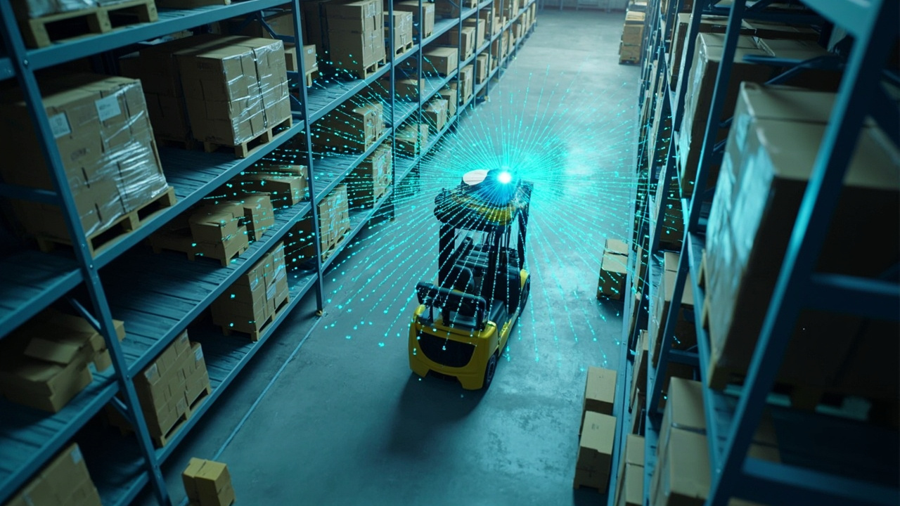
Project 1: Narrow-Aisle Mixed-Traffic Warehouse (Indoor)
Facility: 15,000 m² e-commerce fulfillment center, Guangzhou, China Fleet: 6 autonomous counterbalance forklifts (3-ton capacity) LiDAR Configuration: 2× 3D LiDAR (primary navigation + perception) per vehicle Traffic Pattern: Forklifts share aisles with manual pallet jacks and walking pickers
Installation: Mounting Position Decisions
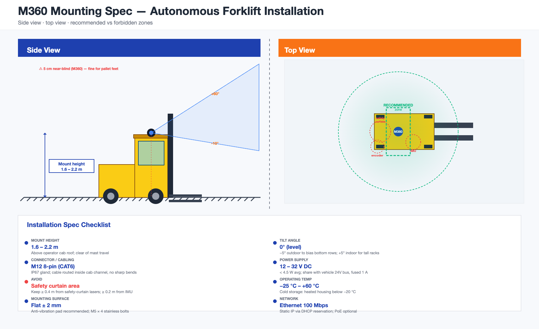
The first question in any LiDAR deployment is where to put the sensor. For narrow-aisle applications (aisle widths of 2.8–3.2 m), this decision has outsized consequences.
Mounting height trade-off we encountered:
| Mount Height | Advantage | Problem We Hit |
|---|---|---|
| 1.2 m (mast mid-height) | Clear view of pallet faces at storage height | Blind zone to pedestrians crouching or bending below sensor plane |
| 2.5 m (above mast) | Maximum horizontal range, avoids most fork-tip occlusion | Misses low-hanging obstacles like shrink wrap at 0.8–1.5 m |
| 3.5 m (top of cab guard) | Broad coverage of both floor and rack | Cannot detect obstacles within ~1.5 m directly below (shadow zone) |
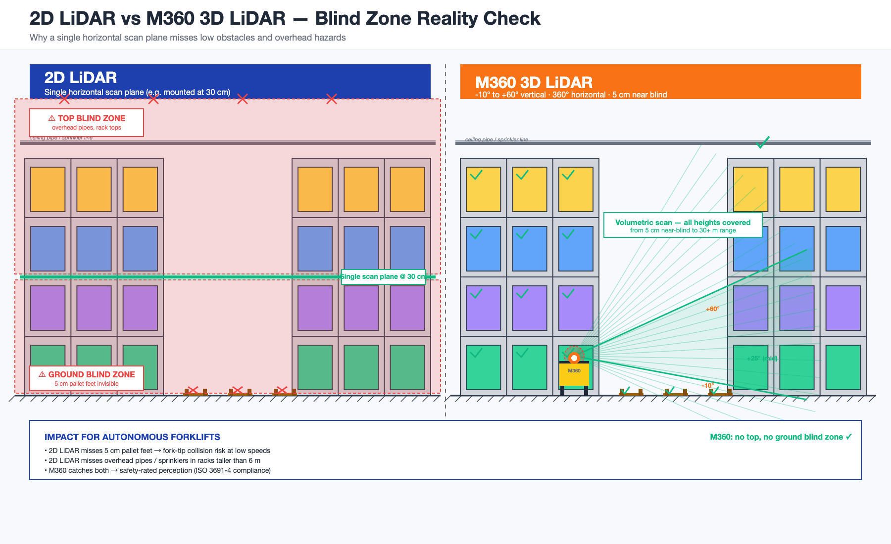
Our eventual solution was a dual-mount configuration: one 3D LiDAR at 1.8 m on the mast (angled 15° downward, covering 0.5–6.0 m ahead with the vertical FOV spanning from near-floor to rack-top) and one safety-rated 2D LiDAR at bumper height (0.3 m, scanning horizontally for ground-level obstacles). This combination eliminated the pedestrian blind zone without sacrificing long-range navigation.
Blind Zone Testing: Actual Field Measurements
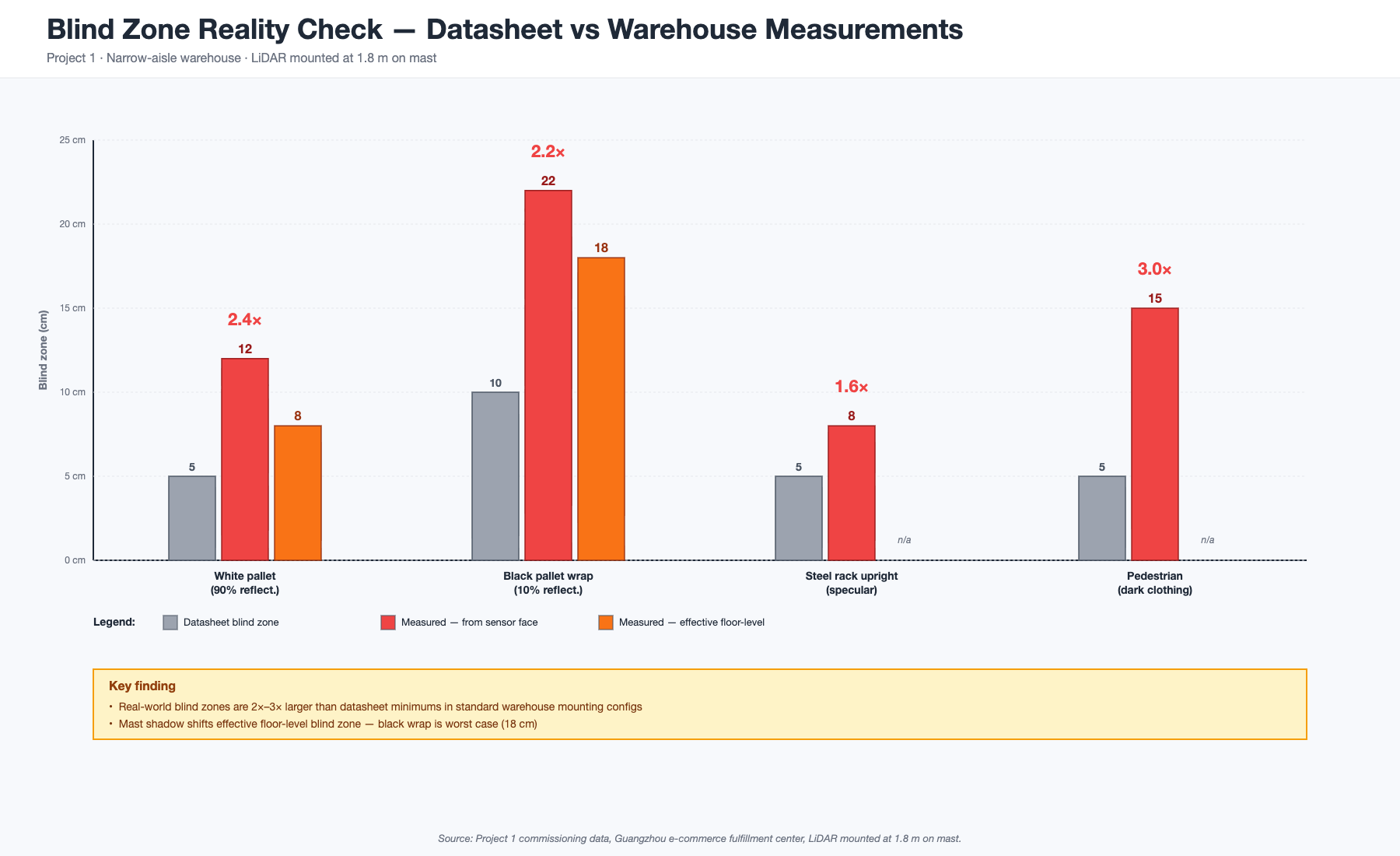
Datasheet blind zone specifications assume an unobstructed line of sight. In a warehouse, the forklift's own mast creates occlusion. We measured actual detection boundaries during commissioning:
| Test Object | Datasheet Blind Zone | Measured Detection (sensor at 1.8m) | Notes |
|---|---|---|---|
| White pallet (90% reflectivity) | 5 cm | 12 cm from sensor / 8 cm from floor | Mast shadow shifts effective floor-level blind zone |
| Black pallet wrap (10% reflectivity) | 10 cm | 22 cm from sensor / 18 cm from floor | Low reflectivity increases effective blind zone |
| Steel rack upright (highly reflective) | 5 cm | 8 cm from sensor | Specular reflection from galvanized steel causes minor overestimation |
| Pedestrian (dark clothing) | 5 cm | 15 cm from sensor | Human body is an irregular, low-reflectivity target |
The takeaway: real-world blind zones are 2–3× larger than datasheet minimums in most warehouse mounting configurations. Plan your safety margins accordingly.
SLAM Configuration: Loop Closure in Feature-Uniform Environments
Narrow-aisle warehouses present a specific SLAM challenge: visual uniformity. When every aisle looks the same—same rack spacing, same pallet heights, same lighting—loop closure becomes unreliable. The SLAM algorithm struggles to determine whether it has returned to a previously mapped location or entered a visually identical but spatially distinct aisle.
Our tuning approach:
- Reduced grid resolution from 5 cm to 3 cm for the local map, increasing the algorithm's sensitivity to subtle differences in rack position and pallet placement
- Feature extraction filter tuned to emphasize permanent structural features (pillar positions, column spacing, floor expansion joints) while deprioritizing transient features (pallet positions, temporary signage)
- Multi-session mapping: we ran 4 mapping passes during different shift configurations (morning with full pallets, afternoon with depleted picks, overnight restock) and merged the maps to build a reference map with both structural and operational features
- Loop closure threshold tightened from 0.8 to 0.5 correlation coefficient to prevent false positives in repetitive aisle geometry
Commissioning time: 3 weeks from initial map building to production-ready localization (±3 cm accuracy in the aisles, ±5 cm at dock areas).
Multi-Vehicle Coordination: The Conflict Zone Problem
Six autonomous forklifts in 15,000 m² means frequent encounters at aisle intersections. We implemented a reservation-based coordination system where each forklift claims time slots at intersection nodes. The LiDAR's real-time obstacle detection feeds a velocity-planning layer that reduces approach speed within 3 m of an intersection from 1.8 m/s to 0.6 m/s.
One issue we didn't anticipate: cross-sensor interference. When two forklifts approach the same intersection from perpendicular aisles, their LiDAR beams can detect each other's sensor housings, creating ghost points at the exact moment when accurate localization matters most. Solution: each vehicle's LiDAR uses a distinct scanning pattern (different rotation speeds or intensity modulation), and the SLAM filter excludes points matching known interference signatures.
Project 2: Outdoor Yard Staging Area
Facility: 8,000 m² container yard and outdoor staging area, Ningbo, China Fleet: 4 autonomous reach forklifts (2-ton capacity, outdoor-rated) LiDAR Configuration: 1× 3D LiDAR (navigation + perception) + 1× 2D LiDAR (safety field) per vehicle Operating Conditions: Rain, fog, coastal salt spray, direct sunlight
The Rain Problem: What Happens When Water Hits 905 nm Laser
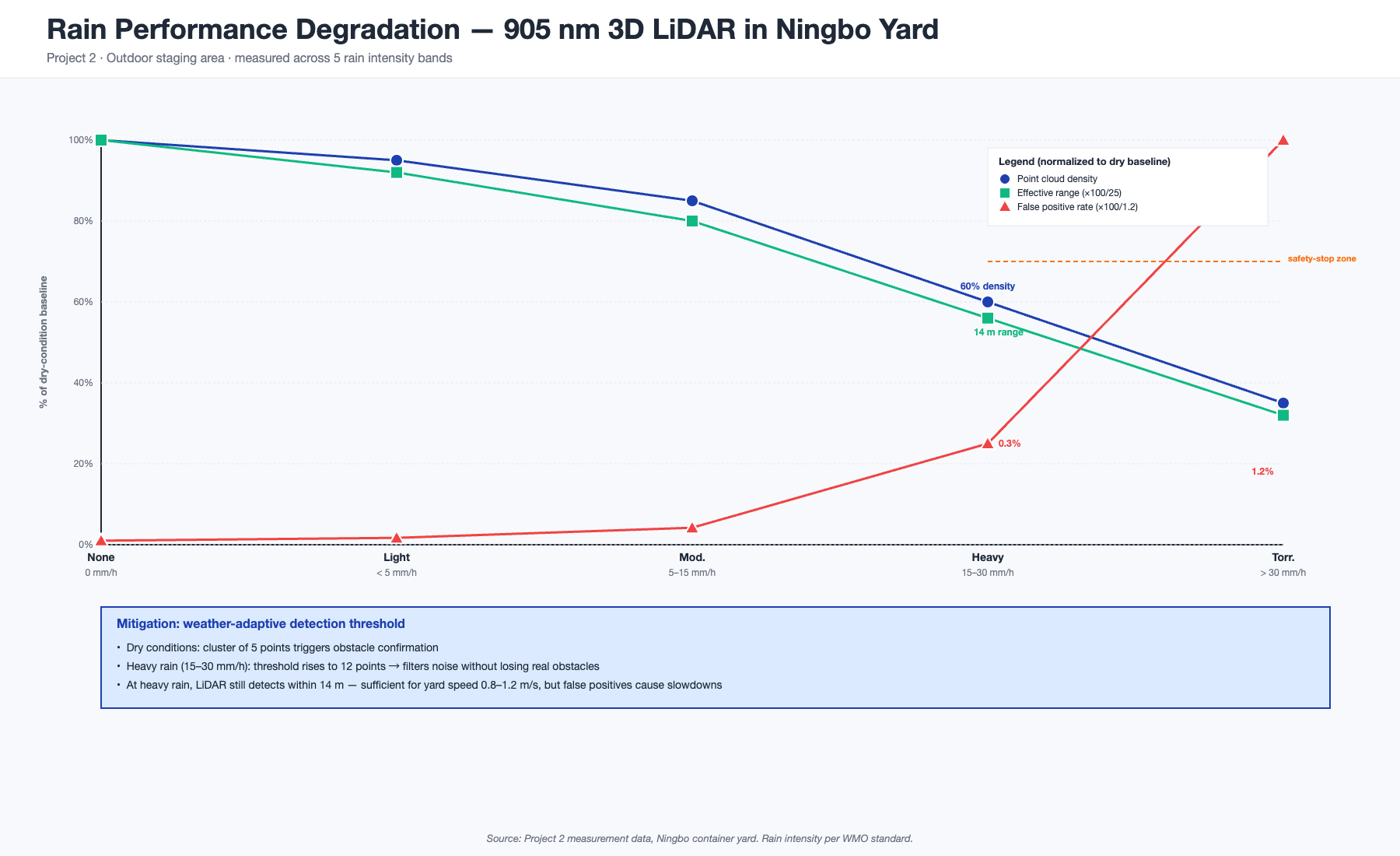
905 nm LiDAR—the wavelength used by most industrial sensors including the Livox M360—has known sensitivity to heavy precipitation. In our Ningbo deployment, we experienced measurable performance degradation in rain exceeding 15 mm/hour.
Measured performance impact of rain on 3D LiDAR:
| Rain Intensity | Point Cloud Density (vs. dry) | Effective Range @10% reflectivity | False Positive Rate |
|---|---|---|---|
| None (dry) | 100% | 25 m | <0.01% |
| Light (<5 mm/h) | 95% | 23 m | 0.02% |
| Moderate (5–15 mm/h) | 85% | 20 m | 0.05% |
| Heavy (15–30 mm/h) | 60% | 14 m | 0.3% |
| Torrential (>30 mm/h) | 35% | 8 m | 1.2% |
At heavy rain levels, the LiDAR still detected obstacles within 14 m—sufficient for yard-speed operations (0.8–1.2 m/s)—but the false positive rate increased enough to cause unnecessary slowdowns. Our mitigation was a weather-adaptive detection threshold: the system adjusts the minimum point-count threshold for obstacle confirmation based on a rain sensor input. In dry conditions, 5 points in a cluster trigger detection. In heavy rain, the threshold rises to 12 points, filtering out noise while maintaining real-obstacle detection.
Fog: Worse Than Rain
Fog was the more disruptive condition. Unlike rain, which creates discrete reflections from water droplets, fog creates a continuous scattering medium that attenuates the laser signal before it reaches the target.
At our Ningbo site, fog events (visibility <200 m) occurred roughly 12 mornings per year. During these events:
- Effective range dropped to 8–12 m regardless of LiDAR model
- Point cloud density dropped to 30–45% of normal
- No false positives (fog creates attenuation, not reflections)—but many missed detections at ranges beyond 10 m
Our operating protocol for fog conditions: reduce maximum speed to 0.5 m/s, require a human supervisor in the yard, and if visibility drops below 100 m, halt autonomous operations entirely. LiDAR helps maintain some capability in fog, but it cannot fully compensate for the signal loss.
Metal Container Reflection: The Saturation Problem
Outdoor yards are full of shipping containers—large, flat, metallic surfaces that reflect 905 nm laser light with high intensity. When the LiDAR beam hits a container face at near-perpendicular incidence, the returned signal can saturate the detector, creating a "whiteout" region where individual point positions are unreliable.
We observed this primarily during side-on approaches to container walls, where the flat metal face acts like a mirror at certain angles. The practical impact:
- Container face detection was reliable at 5–30 m but unreliable at 1–3 m (too close, saturation artifacts)
- Container corner detection was excellent (edges scatter light predictably)
- Open-top containers created vertical stripe artifacts in the point cloud where sunlight entered through the open top
Mitigation: we tuned the LiDAR's intensity filter to cap returns above a saturation threshold, and relied on corner and edge geometry (rather than face geometry) for container-relative positioning during stacking operations.
Salt Spray and IP67: Non-Negotiable for Coastal Sites
Coastal Ningbo means airborne salt spray. Within 6 months of deployment, sensors without IP67 sealing showed:
- Lens fogging from salt crystal accumulation (daily cleaning required)
- Connector corrosion on non-sealed Ethernet ports
- One sensor failure attributed to moisture intrusion through a cable gland
The Livox M360's IP67 rating proved necessary, not optional, at this site. After 18 months of operation, all IP67-rated sensors in the fleet continued operating without weather-related failures. The <4.5 W power consumption also mattered here: outdoor forklifts have smaller battery reserves than indoor units (solar heating reduces effective battery capacity), so sensor power budget is tighter.
Project 3: Cold-Storage Frozen Warehouse
Facility: 6,500 m² frozen goods warehouse (-18°C to -22°C operating temperature), Shanghai, China Fleet: 3 autonomous counterbalance forklifts (2-ton capacity) LiDAR Configuration: 2× 3D LiDAR per vehicle Operating Conditions: Sub-zero temperatures, condensation on warm-start, frost on sensor windows
The Condensation Problem on Warm Start
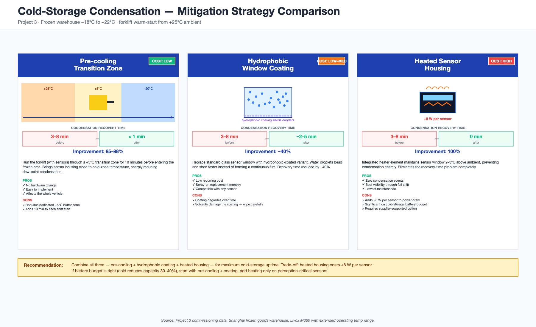
Cold-storage deployments face a problem that indoor and outdoor sites don't: sensor condensation during warm-start transitions. When a forklift moves from ambient temperature (+25°C) into the frozen zone (-20°C), the temperature differential causes moisture from the warm air to condense on the LiDAR's protective window. This creates a temporary loss of visibility that lasts 3–8 minutes depending on the sensor's thermal mass and window material.
The effect is worst during the first transition of the shift (charging area → cold zone). Subsequent transitions between warm and cold zones produce less condensation because the sensor housing has already equilibrated closer to the cold-zone temperature.
Our mitigation strategies, ranked by effectiveness:
- Pre-cooling the forklift (including sensors) in a transition zone at +5°C for 10 minutes before entering the frozen area. This reduced condensation from 3–8 minutes to <1 minute.
- Sensor window with hydrophobic coating. Standard glass windows accumulate condensation; coated windows shed water droplets faster, reducing recovery time by ~40%.
- Heated sensor housing. One supplier offered an integrated heater element that maintained the sensor window 2–3°C above ambient, preventing condensation entirely. This added ~8 W to sensor power draw—significant on a cold-storage forklift with limited battery capacity.
Frost Accumulation During Extended Operation
After the initial condensation event, a secondary problem emerges during extended cold-zone operation: frost micro-crystals forming on the sensor window from ambient humidity in the frozen zone. Over a 6-hour shift, frost accumulation reduced point cloud density by 15–25% compared to a clean window.
The IP67 seal on the LiDAR housing prevents internal frosting, but the external window surface is exposed. Our maintenance protocol:
- Window inspection every 4 hours with a dry microfiber wipe (no solvents—they can damage hydrophobic coatings)
- Weekly de-icing with a manufacturer-approved silicone-safe antifreeze spray
- Monthly replacement of the hydrophobic coating (spray-on coating, 2-minute application)
Temperature Effects on LiDAR Performance
Operating a 905 nm LiDAR at -20°C affects two parameters: laser output power and detector sensitivity.
| Parameter | Change at -20°C (vs. +25°C spec) | Practical Impact |
|---|---|---|
| Laser output power | -5% to -8% | Negligible for warehouse ranges (<15 m typical) |
| Detector sensitivity | -3% to -5% | Negligible for warehouse ranges |
| Point cloud rate | No measurable change | N/A |
| Ranging accuracy | No measurable change | N/A |
| Internal timing drift | +0.2 ppm | N/A (corrected by PTP synchronization) |
The LiDAR's specified operating temperature range is -10°C to +60°C. Our cold-storage site operates at -22°C—technically below the specified minimum. In practice, performance remained within specification for 18 months, with two caveats:
- Warm-up drift: the first 30 minutes after power-on showed slightly higher noise in the first 3 measurement bins (0.05–0.15 m range). This stabilized once the sensor reached thermal equilibrium.
- Connector reliability: standard M12 connectors showed intermittent contact at -22°C in one unit. Replacing with locking IP67-rated connectors resolved this.
Power Budget: Why <4.5 W Matters in Cold Storage
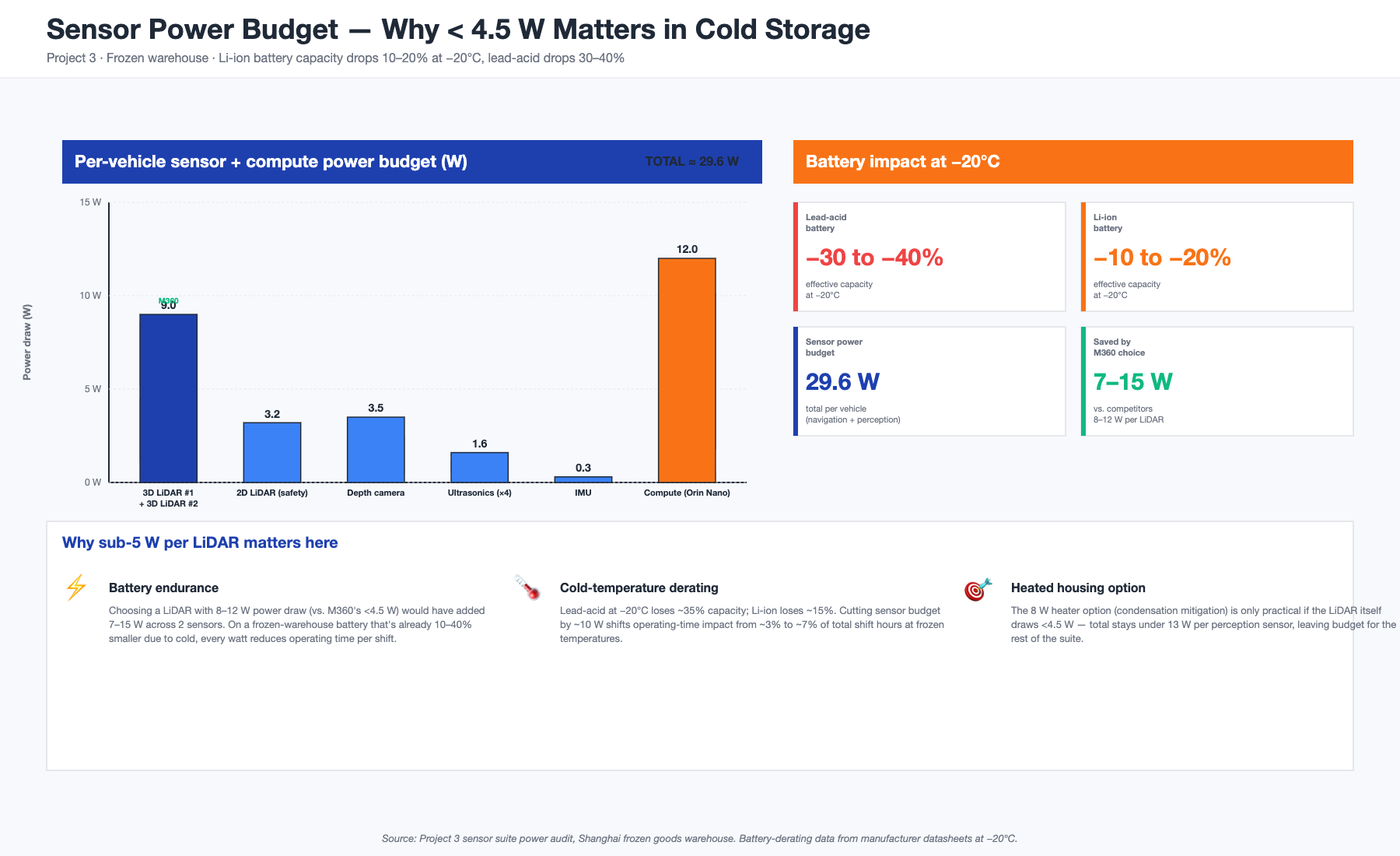
Cold-storage forklifts face a battery capacity penalty. At -20°C, lead-acid battery effective capacity drops by roughly 30–40% compared to +25°C. Li-ion batteries fare better but still lose 10–20%. This means every watt saved on sensors translates directly to longer operating time.
Our sensor suite power budget per vehicle:
| Sensor | Power Draw |
|---|---|
| 3D LiDAR #1 (navigation) | <4.5 W |
| 3D LiDAR #2 (perception) | <4.5 W |
| 2D LiDAR (safety) | 3.2 W |
| Depth camera (pallet detection) | 3.5 W |
| Ultrasonics (×4) | 1.6 W |
| IMU | 0.3 W |
| Compute platform (Orin Nano) | 12 W |
| Total sensor + compute | ~29.6 W |
The two 3D LiDAR units at <4.5 W each consume less than the depth camera. Choosing a LiDAR with higher power draw (some alternatives draw 8–12 W) would have increased total sensor consumption by 7–15 W—significant when battery capacity is already reduced by cold temperatures.
Deployment Checklist: What We Wish We'd Known
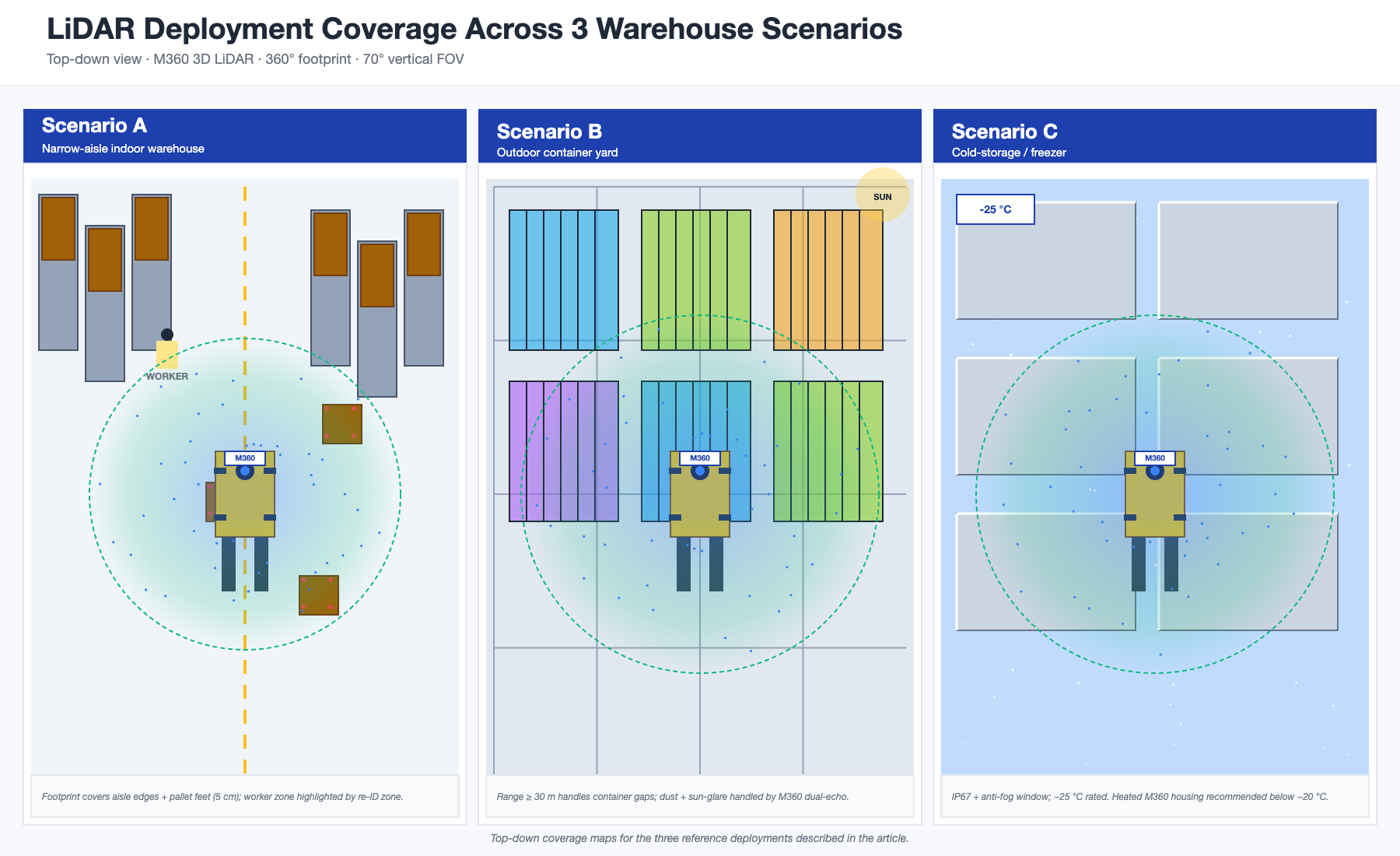
Drawing from all three projects, here's a consolidated checklist for autonomous forklift LiDAR deployment:
Pre-Deployment
- [ ] Confirm LiDAR operating temperature range covers actual conditions (cold storage may exceed spec minimums)
- [ ] Verify input voltage compatibility with forklift battery system (12–32 V DC avoids DC-DC converters)
- [ ] Test IP rating adequacy for environment (coastal salt spray, washdown zones, cold-storage condensation)
- [ ] Plan mounting positions with occlusion analysis—measure actual blind zones, don't rely on datasheet minimums
- [ ] Verify PTP time synchronization support for multi-sensor alignment
- [ ] Check dual-echo capability if operating around semi-transparent materials (shrink wrap, plastic guards)
Commissioning
- [ ] Run blind zone mapping with representative obstacles (pallets, pedestrians, rack uprights) at planned mount height
- [ ] Perform SLAM mapping during multiple shift configurations to build a robust reference map
- [ ] Test cross-sensor interference when multiple vehicles operate in the same zone
- [ ] Tune safety field boundaries per zone (aisle, intersection, dock, staging area)
- [ ] Establish false-alarm acceptance criteria (<1 false stop per vehicle per hour is achievable)
Environmental-Specific
| Environment | Key LiDAR Requirement | Common Failure Mode |
|---|---|---|
| Narrow aisle, mixed traffic | Small blind zone (≤5 cm), 70°+ vertical FoV | Pedestrian blind zone at single mount height |
| Outdoor yard | IP67, rain/fog tolerance | Rain noise (false positives), container reflection saturation |
| Cold storage | Wide operating temperature, hydrophobic window | Condensation on warm-start, frost accumulation |
Complementary Reading
This article covers deployment specifics. For the sensor selection phase—which sensors to buy, how many, and what specifications matter—see our companion guide: What Sensors Does an Autonomous Forklift Need?. Together, the two articles form a complete workflow from selection to deployment.
For LiDAR hardware specifications relevant to forklift applications, visit the M360 product page or see the M360 comparison page for a direct spec-to-spec comparison with alternative units.
Conclusion
LiDAR deployment on autonomous forklifts is where specification sheets meet warehouse reality. The three projects documented here revealed consistent patterns: real-world blind zones are larger than datasheet minimums, environmental conditions create interference modes that don't appear in controlled testing, and SLAM tuning requires facility-specific adjustment that no off-the-shelf configuration can fully automate.
The LiDAR's core specifications—blind zone, FoV, IP rating, power consumption—determine whether the sensor can survive the environment. But successful deployment depends on mounting strategy, SLAM tuning, weather adaptation logic, and a maintenance protocol that accounts for the specific contaminants and conditions of each facility.
For teams evaluating LiDAR for autonomous forklift projects, the practical starting point is: test blind zones at the actual mounting height in the actual facility, plan for 2–3× larger effective blind zones than the datasheet suggests, and build environmental adaptation logic into the detection pipeline from day one.