LiDAR for Tunnel and Underground Infrastructure Inspection

A tunnel engineer walks through a 4-kilometer highway bore at 2 a.m., flashlight in one hand, crack gauge in the other. She marks spalling on the lining with spray paint, photographs the worst sections with a DSLR, and fills out a paper form. Two shifts to cover the corridor. Three months later, half the crack measurements don’t align with the previous inspection cycle because two different inspectors held the gauge at slightly different angles.

This scenario still plays out across much of the world’s underground infrastructure. Photogrammetry helped. You could stitch photos into ortho-mosaics. But it collapses under tunnel lighting conditions: dark, uneven, reflective surfaces, wet concrete, headlight glare. Even with clean images, photogrammetry struggles to deliver the sub-millimeter geometric precision engineers need for crack width quantification and deformation analysis.

LiDAR changes the arithmetic. Instead of measuring how surfaces look, it measures where they are. Millions of XYZ coordinates per second, indifferent to illumination, indifferent to contrast. For underground structures where conventional surveying is slow, unsafe, or simply inaccurate, laser scanning has become the default approach in TBM tunnels, utility vaults, mine galleries, and metro systems.

Why conventional tunnel inspection falls short

Manual visual inspection

Human inspectors still form the backbone of tunnel monitoring in many regions. Walk the tunnel, look for defects, measure what you find. Speed is the obvious problem. A single inspector moving through a 2,000-meter tunnel at walking pace can take 8–12 hours. Safety is the other issue. Standing in a live traffic lane, or beneath unsupported rock in an adit, is never risk-free.

The less obvious issue is reproducibility. Two inspectors measuring the same crack report different widths. Temperature, fatigue, gauge angle all introduce noise. When you’re tracking whether a 2mm crack has widened to 2.3mm over twelve months, ±0.5mm measurement uncertainty swamps your signal.

Photogrammetry and total station surveys

Photogrammetry gives you a photographic record and, with careful geometry control, a 3D reconstruction. Cameras are cheap, processing software is mature. Trouble starts when you try to extract millimeter-scale crack metrics from a photogrammetric model. Geometry depends on texture and contrast, which tunnel linings often lack. Wet concrete, painted markings, uniform grey shotcrete confuse feature-matching algorithms. The resulting point clouds have irregular density and occasional warping.

Total stations deliver high angular and distance accuracy but are painfully slow for full-tunnel coverage. A typical survey crew captures 40–60 discrete points per hour. A tunnel lining needing continuous geometric monitoring requires orders of magnitude more data density than a total station can provide in a reasonable time window.

How LiDAR solves the measurement problem

LiDAR sensors emit laser pulses and record time-of-flight for each return, converting that into distance. Modern sensors output point clouds at 100,000 to 2,000,000+ points per second, each carrying XYZ coordinates and usually an intensity value that reflects surface reflectivity.

For tunnel inspection, a few properties matter more than others.

Point cloud density and precision

A terrestrial LiDAR scanner at the center of a 12-meter-diameter tunnel generates a point every few millimeters on the surrounding lining. At that density, individual cracks with openings as small as 1mm become visible in the point cloud. Not as images, but as geometric discontinuities. You can extract crack width, length, orientation, and depth from the point geometry itself, so measurements aren’t subject to lighting, camera angle, or surface texture.

When the same tunnel is scanned on a six-month cycle, the two point clouds can be registered to a common coordinate frame and subtracted. Differential analysis reveals lining deformation, joint movement, and crack propagation with sub-millimeter resolution.

Active illumination

LiDAR sensors carry their own light source. A tunnel can be completely dark and the scanner still produces high-quality returns off concrete, rock, steel, and water-slicked surfaces. The cost and logistics of illuminating a 3-kilometer tunnel for photography are non-trivial.

The intensity channel adds another dimension. Damp patches on a concrete lining, which show up as subtle tonal changes in a photograph, produce measurable differences in laser return intensity. Analysts use intensity maps alongside geometric data to identify moisture ingress, efflorescence, and delamination zones.

Speed versus manual throughput

A terrestrial laser scanner (TLS) captures a full 360° field of view in 2–6 minutes per station. With setup, repositioning, and overlap, a TLS crew can cover 300–500 meters of tunnel per shift. Mobile systems mounted on vehicles or rail carts push this to several kilometers per hour. Compared to a walking inspector covering 200 meters in an 8-hour shift, the throughput improvement is on the order of 10–50x.

The speed advantage matters operationally. Highway tunnels often have narrow maintenance windows of a few hours between midnight and 5 a.m. Rail tunnels may only be accessible during possession periods of 4–6 hours. When your tool covers the entire tunnel within that window, you avoid staging work over multiple nights. Less traffic disruption, fewer possession costs, faster data turnaround.

From point clouds to BIM

Raw point clouds are geometrically rich but difficult to interpret in isolation. The real value emerges when point cloud data is processed into structured models: BIM objects, meshed surfaces, or deformable templates comparing as-built geometry against design specifications.

In practice, this means importing registered point clouds into software that fits cylindrical or elliptical templates to the tunnel cross-section, extracts clearance envelopes, identifies regions where as-built geometry deviates from design, and flags defects against historical baselines. Many tunnel operators now maintain a rolling digital twin: a continuously updated 3D model that incorporates each new scan cycle.

What kinds of tunnel inspections LiDAR supports

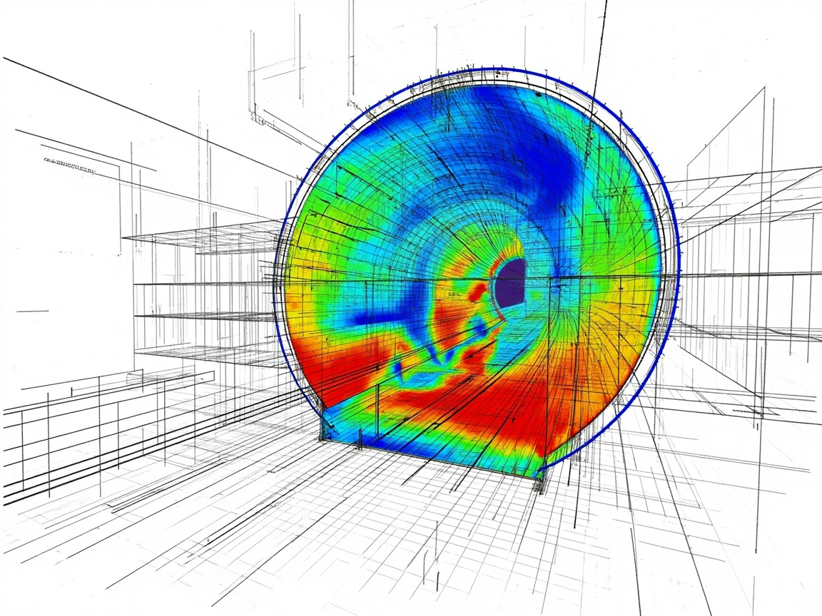
Four inspection tasks show up most often, each with its own precision and coverage requirements.

Clearance profiling is the simplest. Scan the tunnel, fit a nominal cross-section (circular or horseshoe), and flag intrusions into the required envelope. Rail tunnels care about pantograph height and side clearance. Highway tunnels care about lane width and vertical clearance. LiDAR clearance checks typically need 10–20mm absolute accuracy, which mobile or handheld scanners deliver in a single pass.

Lining defect extraction is more demanding. Cracks, spalling, water staining, joint offsets, all requiring millimeter-level resolution on the lining surface. TLS still wins on absolute precision, but mobile scans at close range (under 10 meters from the lining) deliver enough density for crack detection if platform speed is kept low.

Deformation monitoring is a time-series problem. Multiple scan cycles over months or years need registration to a common coordinate frame, and differential analysis reveals gradual change. Requires survey-grade control points and careful registration. TLS is the standard, though some teams are starting to use high-grade mobile scanners for sub-5mm relative deformation tracking.

Lining condition assessment combines the above with material condition data (often from photogrammetry or thermal imaging) into a single asset rating. LiDAR provides the geometric backbone; complementary sensors add the material story.

SLAM in tunnels: why it’s hard and how to make it work

Most mobile and handheld LiDAR systems rely on SLAM (Simultaneous Localization and Mapping) for trajectory estimation when GPS is unavailable. In tunnel environments, SLAM faces three specific challenges.

Geometric degeneracy. A long, straight tunnel with a uniform circular cross-section looks nearly identical to itself at any point along its length. SLAM algorithms that depend on feature matching get confused because there are no distinctive features to match. The algorithm can drift along the tunnel axis without realizing it.

GPS denial. Tunnels block all GNSS signals. Without satellite positioning, the system depends entirely on inertial and LiDAR odometry. IMU drift accumulates over time.

Lighting transitions. The area near tunnel portals has rapid light transitions, from bright daylight to complete darkness within a few meters. For visual-inertial SLAM systems (cameras alongside LiDAR), these transitions can cause tracking failures. Pure LiDAR SLAM is more tolerant since it doesn’t depend on lighting.

The standard mitigation for degeneracy is to inject known control points. For longer tunnels where installing targets is impractical, a hybrid approach combining LiDAR SLAM with periodic loop closures helps bound drift.

A more recent approach is to use LiDAR-inertial odometry (LIO) algorithms such as FAST-LIO2, which tightly couple the LiDAR scans with IMU measurements to estimate motion. FAST-LIO2 is well-suited to tunnel work because it can maintain tracking even during rapid motion or temporary feature scarcity. Pairing FAST-LIO2 with a LiDAR that has an integrated 6-axis IMU produces the cleanest results: timestamps are aligned, and the algorithm uses both data streams directly without external synchronization.

For practical tunnel scanning, a common configuration is a 360° LiDAR sensor running FAST-LIO2 on a small onboard computer, with the sensor head mounted on a handheld pole or backpack frame. The operator walks through the tunnel at steady pace, the system records the raw point cloud and IMU data, and post-processing generates the registered map.

Scanning approaches: stationary, mobile, and handheld

The choice depends on tunnel geometry, precision requirements, access time, and budget.

Stationary (tripod-mounted) terrestrial laser scanning

A high-precision TLS such as a Leica RTC360, Trimble X7, or Riegl VZ-400 mounts on a tripod at fixed positions along the tunnel alignment. Each scan station captures a full 360° hemisphere with millimeter-level point spacing at ranges of 20–40 meters. Setup per station takes 3–5 minutes; data collection 2–6 minutes. Station spacing depends on required point density and tunnel geometry, typically 15–30 meters in a standard highway tunnel.

The advantage is precision. With survey-grade control points and careful registration, multi-station point clouds achieve global accuracy better than 5mm RMS. This makes TLS the go-to choice for deformation monitoring.

The disadvantage is speed. A 3-kilometer tunnel scanned at 20-meter station spacing requires 150 stations. Even at 5 minutes per station, that’s over 12 hours of instrument time. For one-off surveys or annual inspections, this is manageable.

Mobile scanning (vehicle- or cart-mounted)

Mobile mapping systems combine one or more LiDAR sensors with a GNSS/INS unit. The platform moves continuously through the tunnel while sensors collect data, and the trajectory stitches the scans into a single registered point cloud.

In tunnels, GNSS signals are unavailable, so the system relies entirely on the IMU, sometimes supplemented by SLAM algorithms. Drift accumulates over distance. Absolute accuracy typically runs 10–30mm; relative accuracy within a single pass is much better, often 5–10mm.

Speed is the main benefit. A vehicle-mounted system moving at 20–30 km/h can scan several kilometers in a single pass. Even a slow-moving cart (3–5 km/h) outpaces stationary scanning.

Handheld and backpack scanning

Handheld laser scanners such as the Leica BLK2GO or GeoSLAM ZEB series let inspectors walk through a tunnel and capture 3D data without stopping. Power on, walk, walk back to close the loop for better SLAM registration, then process.

These systems trade precision for flexibility. Point density on the lining is lower than TLS, typically 10–30mm spacing, and absolute accuracy runs 15–30mm. But for rapid condition assessment, clearance verification, or documenting specific defect locations, handheld scanners fill a useful niche.

They shine in spaces where vehicles can’t go: narrow service galleries, manhole entry shafts, utility vaults, and tunnel portals. A handheld scanner can capture a 500-meter gallery in 15–20 minutes. For deeper tradeoffs between handheld SLAM scanning and tripod-mounted surveying, see our handheld vs terrestrial scanner comparison.

Where LiDAR tunnel inspection actually gets used

Metro and urban rail tunnel inspection

Metro systems in cities like Shanghai, Beijing, Hong Kong, and Singapore run regular inspection cycles on their tunnel networks, typically every 6–12 months. The work happens during off-hours in narrow possession windows. A crew can scan several kilometers of running tunnel during a 4-hour night window, then turn the data around for analysis the next day. Practical challenges: tight clearances, mixed geometries, and integrating scan data with maintenance records that may go back decades.

Highway tunnel disaster monitoring

Highway tunnels, particularly in alpine or seismically active regions, need post-event inspection after earthquakes, floods, or fire. The goal is to confirm the tunnel is safe for traffic before reopening. LiDAR delivers a fast, objective geometric record that can be compared against the pre-event baseline to identify new deformation, debris, or lining damage. Several major highway authorities (EU, Japan, parts of China) now mandate post-event LiDAR scanning as part of their tunnel reopening procedures.

Mine gallery scanning

Mining operations use LiDAR for stope mapping, cavity monitoring, and drift profiling. The environment is harsh: dust, vibration, limited visibility. Exactly where LiDAR’s active sensing and lighting independence pay off. Scanning data helps engineers calculate volume changes between excavation rounds and monitor ground convergence. For a closer look at mining applications, see our mining LiDAR article.

Underground parking and utility corridors

Below-grade parking garages deteriorate in ways less visible than above-ground structures. Water infiltration, de-icing salt exposure, and freeze-thaw cycling cause concrete spalling and reinforcement corrosion. LiDAR scanning captures ceiling and column geometry at millimeter resolution, making it possible to track crack development over time without closing the facility. Combined utility corridors carrying power, water, gas, and telecom lines also benefit: a single LiDAR pass maps the full cross-section including embedded utilities and cable trays.

Data processing: from raw returns to actionable reports

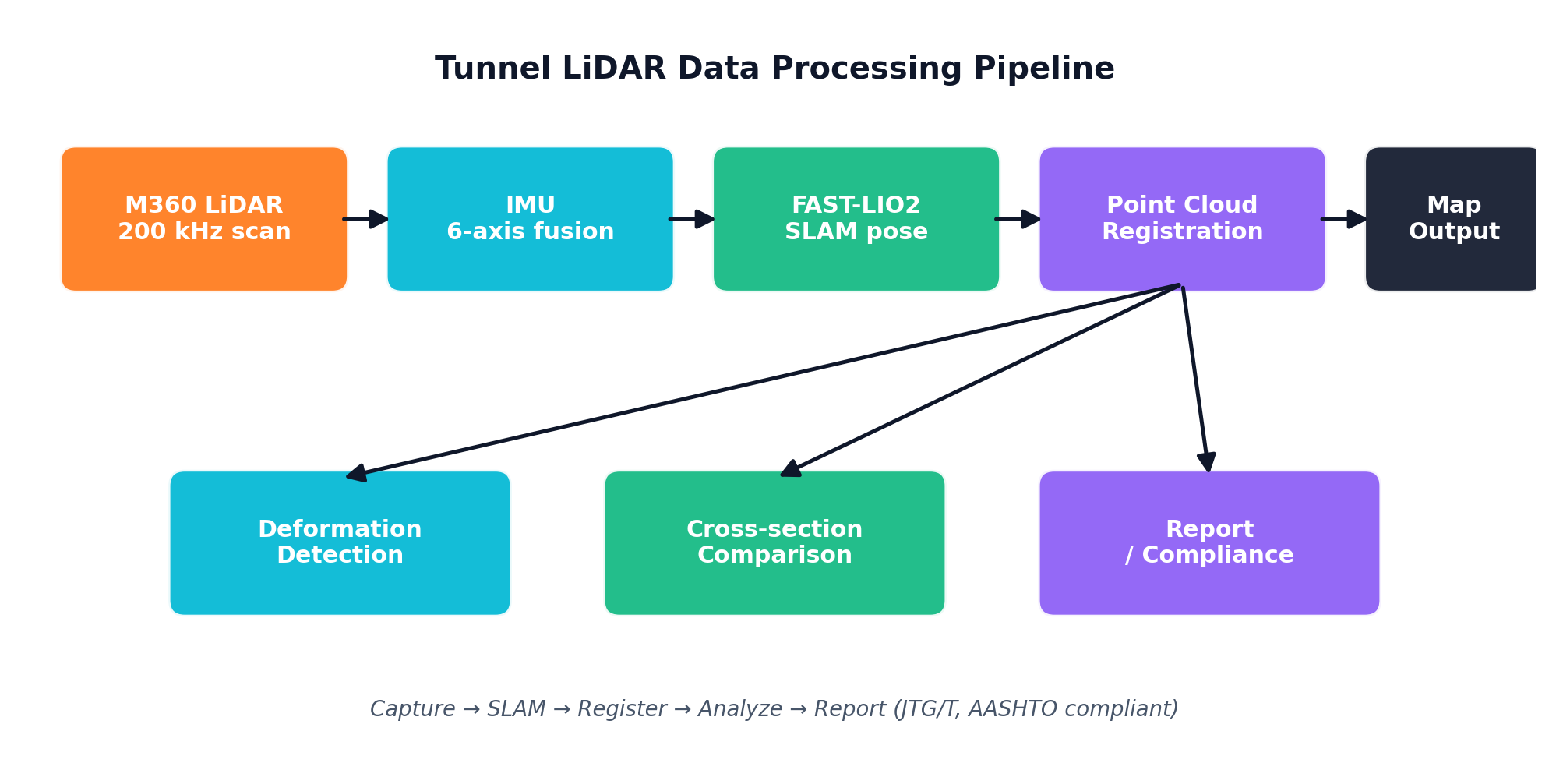
Going from a raw point cloud to an inspection report involves several processing steps.

Noise filtering removes outliers from dust particles, reflective surfaces, and multi-path returns. Statistical outlier removal filters, radius-based methods, and manual clipping clean the data before downstream analysis.

Registration. Multi-station TLS data is registered using target-based (spheres or flat targets) or target-free (cloud-to-cloud ICP) methods. Mobile and handheld systems rely on SLAM-based registration during capture, with optional post-processing refinement using algorithms like FAST-LIO2.

Model fitting aligns the registered point cloud to the nominal tunnel geometry (cylinder, ellipse, or horseshoe profile), calculating deviations between actual lining and design profile at every cross-section. This step generates clearance envelopes and flags local intrusions.

Segmentation divides the point cloud into structural elements: lining, joints, ductwork, cable trays, road surface, fixtures.

Defect extraction. Crack detection algorithms identify geometric discontinuities exceeding configurable thresholds.

Deviation analysis and reporting. When two or more scan epochs are available, differential analysis quantifies deformation, crack propagation, and new defect formation.

Most operators don’t build this pipeline from scratch. Commercial platforms like Bentley iTwin, Autodesk ReCap, and Hexagon Leica Cyclone handle the processing. For custom pipelines, open-source tools like PCL, Open3D, and the FAST-LIO2 stack integrate directly with the LiDAR driver.

Standards and regulatory context

In China, the JTG/T series of standards for highway tunnel maintenance covers inspection cycles, defect classification, and documentation requirements. Mobile and stationary LiDAR scanning are explicitly accepted as inspection methods.

In the US, AASHTO and FHWA publications cover tunnel inspection protocols, though they were written before LiDAR scanning became common. State DOTs are increasingly supplementing manual requirements with their own LiDAR-based programs.

In Europe, the EU tunnel safety directive and various national road authority standards govern highway and rail tunnel inspection. Switzerland, Austria, and Germany have been early adopters of routine LiDAR scanning.

The practical implication: LiDAR scan data can satisfy regulatory reporting requirements, but specific deliverables (defect catalogs, clearance envelopes, deformation curves) need to be formatted according to the local standard.

Selecting the right scanner for tunnel work

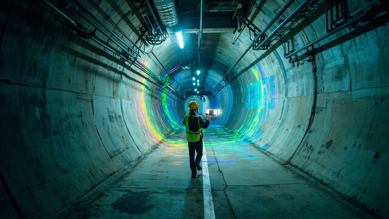
Match the sensor’s capabilities to the constraints of your application.

Match precision to the inspection requirement. Sub-5mm accuracy on a high-speed rail tunnel means stationary TLS is still the benchmark. Corridor-level mapping and clearance checks need only 10–20mm accuracy.

Check the environmental ratings. Tunnels are wet, dusty, and vibration-prone. IP67 isn’t optional for sensors that live on mobile platforms in active tunnels. Operating temperature range matters too.

Evaluate point output rate against platform speed. A sensor running at 200 kHz on a mobile platform moving at 5 m/s generates approximately 40 points per meter of travel. Sparse for crack detection but adequate for gross geometry.

Consider the SLAM/IMU situation. For mobile and handheld scanning in GPS-denied tunnel environments, SLAM registration quality depends on the sensor’s built-in IMU and processing software. An integrated 6-axis IMU provides raw motion data for algorithms like FAST-LIO2.

Think about weight and power for handheld work. A handheld or backpack scanner gets carried through kilometers of tunnel. At 408g and under 4.5W power draw, a lightweight 360° sensor runs for hours on a small battery pack.

Think about data management. A single kilometer of tunnel scanned at 5mm point spacing generates tens of gigabytes of raw point cloud data.

For teams integrating LiDAR into a ROS2 stack, whether for tunnel inspection or other applications, see our ROS2 + LiDAR integration guide.

Putting it together

The sensor hardware is mature, the processing tools work, and the ROI case for replacing manual inspection with laser scanning has been demonstrated across enough projects that it’s no longer experimental. The remaining challenges are organizational: establishing scan-to-report workflows, training analysts, building digital twin infrastructure, and convincing budget holders that the upfront investment pays for itself.

For teams evaluating their first LiDAR purchase for tunnel inspection, define the minimum acceptable precision and coverage for your specific application, then work backward to the sensor class and deployment method that delivers those numbers within your access window and budget. If that leads you to a comparison between sensor options, check the M360 vs MID-360 comparison page for a detailed parameter breakdown. For general LiDAR sensor specifications and purchasing options, visit our product page or contact us directly.