Point Cloud Registration: ICP vs NDT vs TEASER++ vs CPD Compared
Two point clouds. One from sensor frame t, another from t+1. Registration finds the rigid transformation (rotation R + translation t) that minimizes distance between corresponding points across both clouds.
That's the one-sentence version. The hard part is defining "correspondence" when you don't know which point in cloud A maps to which in cloud B, when density differs between frames, when 15% of points are noise or occlusion artifacts, and when you need the answer in under 10 ms for real-time SLAM.
This article breaks down four algorithms engineers actually use - ICP, NDT, TEASER++, and CPD - on the axes that matter: accuracy under noise, outlier tolerance, speed on embedded hardware, and memory footprint. No theory dump. Each section covers how the algorithm works, where it fails, and when you'd pick it over the alternatives.
How Registration Algorithms Are Categorized
Before diving into specifics, it helps to know what families exist. Point cloud registration algorithms fall into roughly four camps:
Point-based (ICP family). Treat each point as an independent observation. Find nearest neighbors, compute transformation. ICP, GICP, Point-to-Plane ICP all live here. The original idea dates to Besl and McKay, 1992.
Distribution-based (NDT family). Bin points into spatial cells, fit a probability distribution to each cell. Optimize the transformation that maximizes the sum of point-to-distribution likelihoods. Biber et al., 2003.
Feature-based (SAC-IA, FPCS, Super4PCS). Extract geometric descriptors (FPFH, SHOT) or use 4-point congruent sets to find coarse alignment without point-to-point matching. Useful as a front-end before ICP refinement.
Probabilistic / robust (CPD, TEASER++, GMMReg). Model the alignment problem as probabilistic inference or robust estimation with truncated losses. Handle outliers and, in some cases, non-rigid deformation.
ICP, NDT, TEASER++, and CPD don't cover the full landscape. But they're the four you'll find in production code the most often. Feature-based methods get a brief mention at the end.
ICP: Iterative Closest Point
ICP is the oldest algorithm here, published by Besl and McKay in 1992, and it's still the default in most point cloud libraries (PCL, Open3D). The name describes the method: iterate, find closest points, compute transform, repeat.
Each iteration does four things:
- Match every point in the source cloud to the nearest point in the target cloud
- Reject outlier pairs whose distance exceeds a threshold
- Compute the rigid transformation that minimizes sum of squared distances between matched pairs
- Apply that transformation to the source cloud
Repeat until convergence - translation delta below 0.001 m or iteration count hits a preset limit.
Point-to-Point vs Point-to-Plane vs GICP
Three variants matter in practice.
Point-to-Point ICP is the original. Minimizes Euclidean distance between matched pairs. Converges slowly when clouds are nearly aligned - the gradients flatten out.
Point-to-Plane ICP (Chen & Medioni, 1991) projects error onto the surface normal at the target point. Convergence rate jumps roughly 5-10x. Trade-off: you need surface normals, which means either computing them on the fly or storing them alongside point data.
Generalized ICP (GICP, Segal et al. 2009) treats each point as a small planar patch and computes a covariance matrix that captures local surface geometry. Combines point-to-plane convergence speed with better behavior on curved surfaces.
Other variants worth knowing:
- Symmetric ICP - minimizes error from both source-to-target and target-to-source, reducing bias when clouds differ in density
- Point-to-Distribution ICP - fits a Gaussian to each local neighborhood, handles partial overlap better
- LM-ICP - uses Levenberg-Marquardt instead of linearized SVD for solving the inner minimization. More stable when residuals are large but slower per iteration.
Where ICP Breaks Down
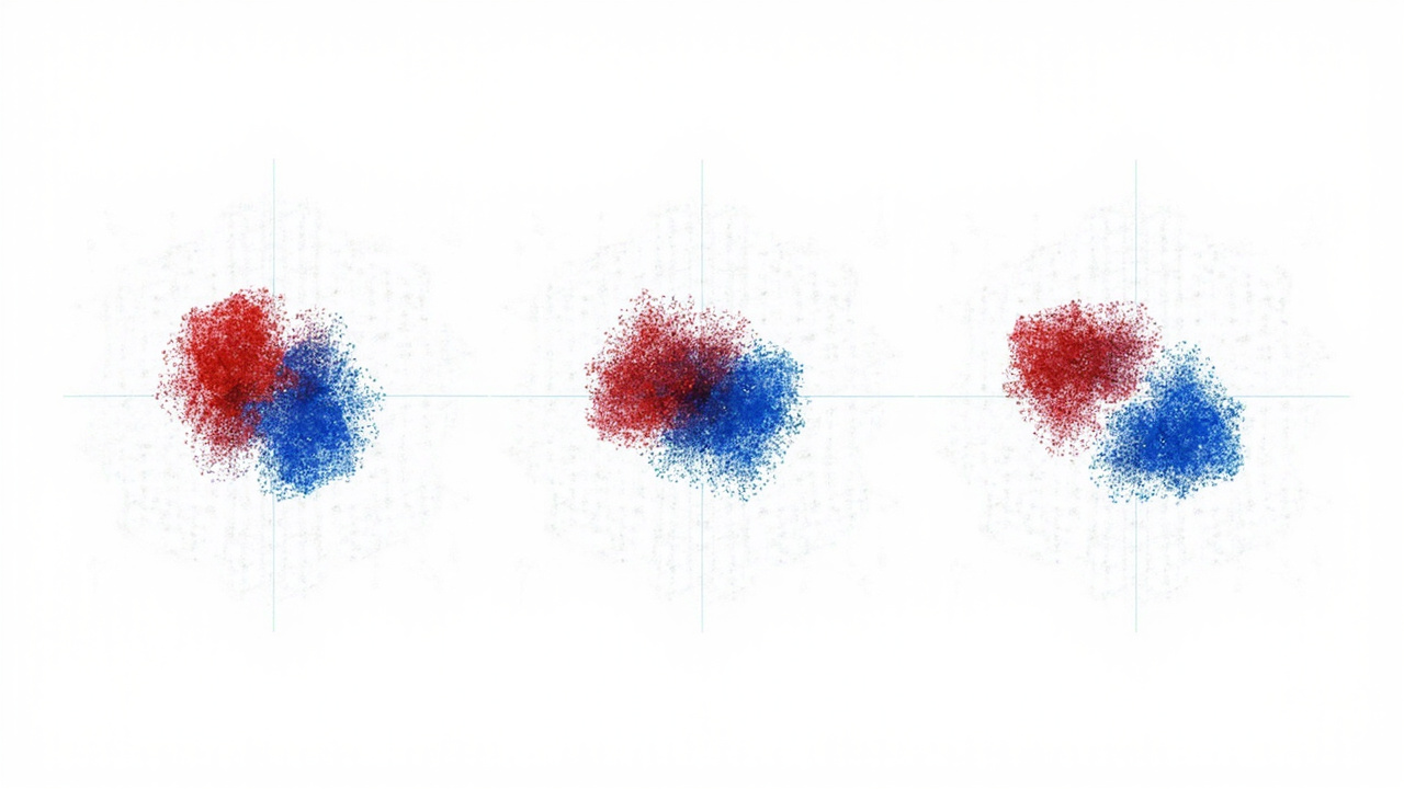
Two failure modes show up constantly in practice.
Local optima. Give ICP a good initial guess (within a few degrees and a few centimeters) and it converges fast. Give it a 30° rotation with no prior and it gets trapped in a local minimum. The result looks plausible but is completely wrong. This is why most ICP pipelines pair it with a coarse pre-alignment step.
Outlier sensitivity. A single spurious point that matches a far-away outlier pulls the entire transformation off. The distance-threshold rejection helps but it's a tuning knob. Too tight and you lose valid matches on surfaces with steep geometry; too loose and outliers corrupt the estimate.
ICP in Open3D
Most engineers using ICP today aren't writing it from scratch - they call it from a library. Open3D's ICP implementation is the easiest to start with:
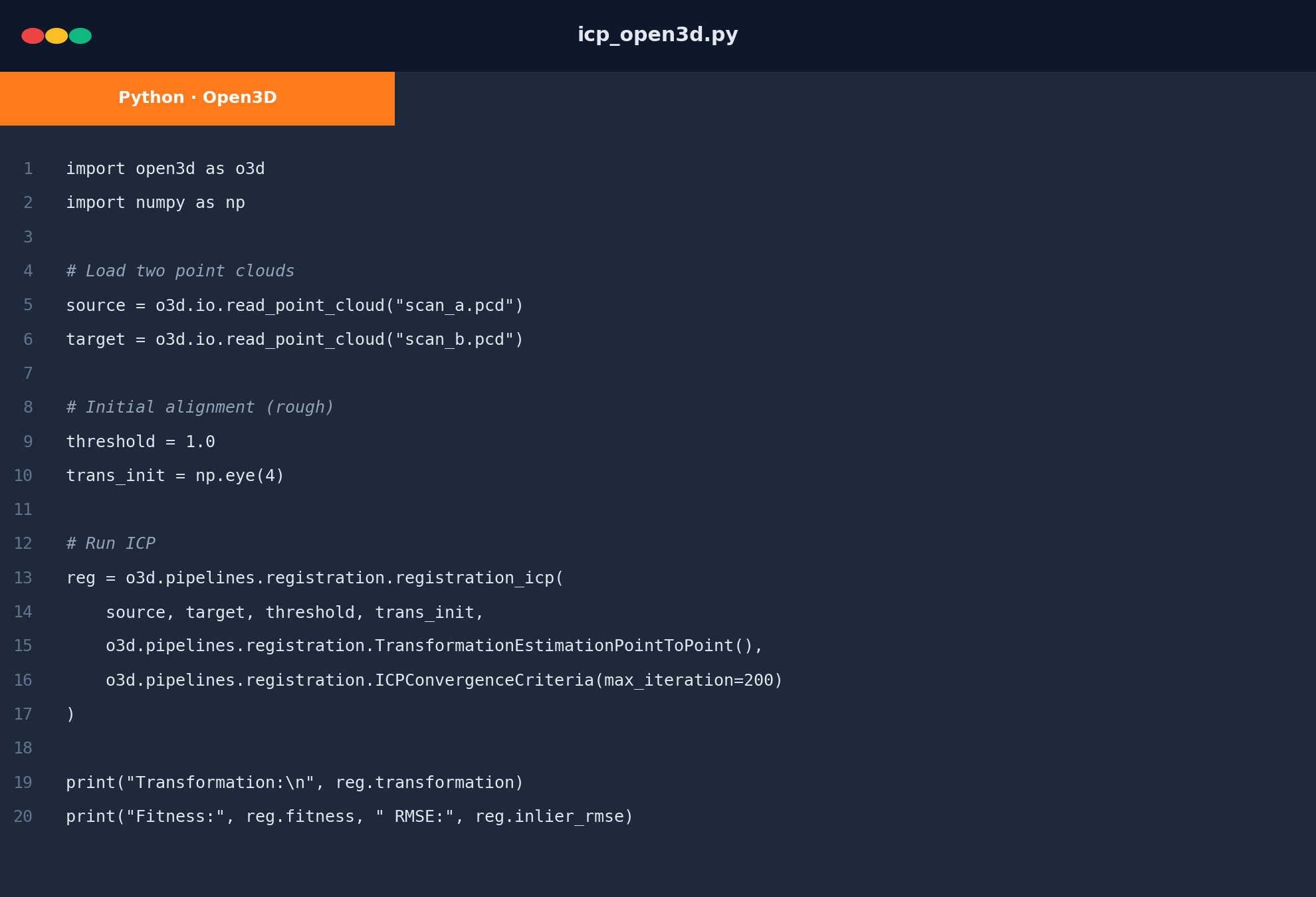
import open3d as o3d

source = o3d.io.read_point_cloud("scan_001.ply")
target = o3d.io.read_point_cloud("scan_002.pcd")

# Initial transformation (e.g., from odometry)
init = np.eye(4)

result = o3d.pipelines.registration.registration_icp(
    source, target,
    max_correspondence_distance=0.05,  # 5cm threshold
    init,
    o3d.pipelines.registration.TransformationEstimationPointToPlane(),
    o3d.pipelines.registration.ICPConvergenceCriteria(max_iteration=50)
)

print(result.fitness_)  # inlier ratio
print(result.inlier_rmse_)
For GICP, swap TransformationEstimationPointToPlane() for TransformationEstimationForGeneralizedICP(). Same call signature, slightly different math under the hood.
Practical numbers: On 50,000-point clouds with good initial alignment (within 2° and 0.5 m), standard ICP converges in 15-30 iterations, taking roughly 50-120 ms on a modern CPU. GICP adds 20-40% overhead but typically reduces final alignment error by 30-50%.
NDT: Normal Distribution Transform
NDT takes a completely different approach. Instead of pairing individual points, it divides the target point cloud into a 3D grid of cells and fits a normal distribution to the points within each cell. Registration then optimizes the transformation that maximizes the likelihood of source points falling within those distributions.
Biber et al. introduced this in 2003, originally for 2D laser scans in mobile robotics. The 3D extension followed naturally.
How NDT Handles Speed
The speed advantage comes from the fixed grid structure. Computing the score for a candidate transformation only requires evaluating which cells the source points land in and summing the Gaussian PDF values. No nearest-neighbor search, no correspondence computation. That makes each evaluation very fast, which matters when you're doing multi-resolution optimization (coarse grid first, then refine).
On a single-threaded CPU, NDT typically runs 3-10x faster than ICP for equivalent point cloud sizes. On GPU implementations, the gap widens further.
The Resolution Sensitivity Problem
NDT's weak point is cell size. Set it too large and each cell captures a big chunk of geometry - the Gaussian becomes a poor fit, you lose detail. Set it too small and cells contain too few points, making the distribution estimate noisy.
Most practitioners run a multi-resolution search: start with a 1-2 m grid for coarse alignment, then refine with 0.5 m and 0.2 m grids. That works, but the parameter tuning doesn't generalize across different environments - an outdoor scene at 50 m range behaves differently from an indoor corridor at 3 m.
NDT in PCL
PCL's NDT registration is straightforward to call from C++:
#include <pcl/registration/ndt.h>

pcl::NormalDistributionsTransform<pcl::PointXYZ, pcl::PointXYZ> ndt;
ndt.setStepSize(0.1);
ndt.setResolution(1.0);  // 1m grid cells
ndt.setMaximumIterations(35);

ndt.setInputSource(source_cloud);
ndt.setInputTarget(target_cloud);

pcl::PointCloud<pcl::PointXYZ>::Ptr output(new pcl::PointCloud<pcl::PointXYZ>);
ndt.align(*output, initial_guess_matrix);

std::cout << "Score: " << ndt.getFitnessScore() << std::endl;
std::cout << "Transform:\n" << ndt.getFinalTransformation() << std::endl;
The setResolution call is where most tuning effort goes. Start at 1.0, drop to 0.5 if you need finer alignment.
NDT in Production
Where NDT shines: large-scale outdoor SLAM. Autonomous driving and agricultural robotics use NDT variants (NDT-OM, multi-layer NDT) for scan matching because the speed advantage at high point counts is significant, and point distributions from vehicle-mounted LiDAR tend to be fairly regular.
A 360° LiDAR producing uniformly distributed points across a wide vertical FOV feeds NDT grids with consistent point density per cell - no region over-saturated, no region starved. If you're comparing LiDAR options for an NDT-based pipeline, see how the M360 stacks up against the MID-360.
Where NDT struggles: structured indoor environments with thin walls and sharp edges. The Gaussian assumption breaks down at planar boundaries, and you get systematic alignment errors near corners.
TEASER++: Trustworthy Estimation Using Semidefinite Relaxation
TEASER++, published by Yang et al. in 2020, takes a fundamentally different path. Instead of iterative local refinement, it formulates registration as a truncated least squares estimation problem and solves it via semidefinite programming (SDP) relaxation.
The Truncated Least Squares Idea
Standard least squares minimizes the sum of squared residuals across all point pairs. One outlier with a 5-meter residual dominates the cost function. Truncated least squares caps the residual contribution - any pair with a distance above a threshold contributes nothing.
The challenge is that the truncated least squares problem is non-convex and hard to solve directly. TEASER++ relaxes it into a semidefinite program (SDP), which is convex and solvable with standard optimization tools. The relaxation is "tight" - the SDP solution is usually identical to or very close to the true optimal.
Why Outlier Tolerance Matters
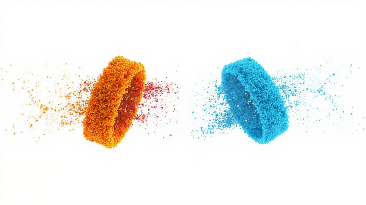
In real-world LiDAR data, outliers come from everywhere. Moving vehicles, glass reflections, rain and fog returns, multipath echoes, and temporal differences between consecutive scans. A scan from a 360° LiDAR outputting points at 200 kHz will inevitably include returns from dynamic objects that don't belong to the static scene geometry.
TEASER++ handles this with its inlier/outlier dichotomy. Each point pair is either accepted (contributes to the cost) or rejected (ignored entirely). There's no soft weighting that lets a borderline outlier partially corrupt the estimate. The algorithm also provides a per-point inlier flag for downstream filtering.
Performance Profile
TEASER++ is slower than both ICP and NDT for well-behaved inputs - the SDP solver has a fixed overhead that doesn't shrink just because your data is clean. Benchmarks on 10,000-point clouds show 30-80 ms per registration on a modern CPU, compared to 5-15 ms for NDT.
On data with significant outliers (20-40% of points), TEASER++ produces dramatically better alignments. ICP and NDT will both fail or produce poor results when outliers exceed roughly 10-15% of the total point count.
This makes TEASER++ the go-to choice for: initial coarse registration (before refining with ICP), loop closure in SLAM, and any application where you can't guarantee clean point clouds.
TEASER++ in Python
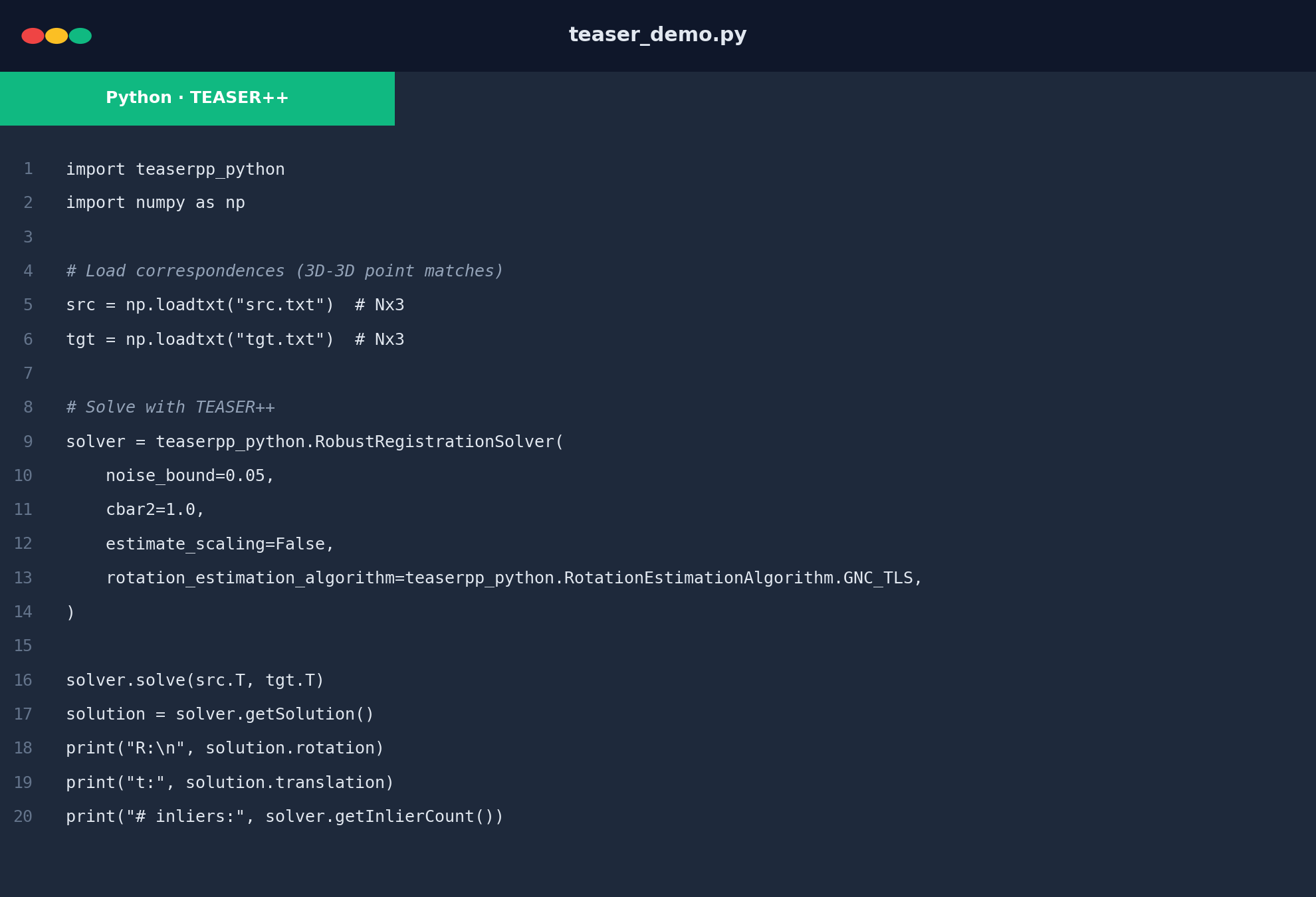
The official teaser-plusplus Python package handles the SDP solving and registration in one call:
import teaserpp_python

# Build solver with truncated least squares estimator
solver_params = teaserpp_python.RobustRegistrationSolver.Params()
solver_params.noise_bound = 0.05  # 5cm noise tolerance
solver_params.estimate_scaling = False
solver_params.cbar2 = 1.0
solver_params.reg_name = "TEASER"

solver = teaserpp_python.RobustRegistrationSolver(solver_params)
solver.solve(src, tgt, correspondences)  # correspondences: Nx2 array of index pairs

solution = solver.getSolution()
print(solution.translation)
print(solution.rotation)
print(solution.inliers)  # boolean mask
The correspondences array is typically produced by a separate feature-matching step (FPFH descriptors, for instance), since TEASER++ doesn't include correspondence search internally.
CPD: Coherent Point Drift
CPD, from Myronenko and Song in 2010, approaches registration from a statistical perspective. It treats the target point cloud as a Gaussian Mixture Model (GMM) centroid set and finds the transformation that aligns the source cloud to this GMM via the Expectation-Maximization (EM) algorithm.
The GMM Framework
Each target point becomes a Gaussian component. The source points are treated as data points generated by this mixture. The EM algorithm alternates between:
- E-step: Compute the probability that each source point was generated by each target component (the "correspondence" matrix)
- M-step: Update the transformation parameters to maximize expected log-likelihood
This naturally handles many-to-one correspondences (multiple source points matching the same target) and provides soft correspondences instead of hard binary matches.
Non-Rigid Registration
CPD's distinguishing feature is support for non-rigid transformations. By adding a displacement field (modeled with a Gaussian Radial Basis Function) on top of the rigid transformation, CPD can align point clouds that have been deformed.
This is relevant in medical imaging - aligning lung CT scans across breathing cycles, registering pre-operative and post-operative brain MRI volumes, matching dental scans. The underlying anatomy moves and deforms, and a purely rigid transformation can't capture the actual correspondence.
Why CPD Rarely Appears in LiDAR Work
For robotics and autonomous systems, the non-rigid capability is mostly irrelevant. Robot chassis don't bend. Buildings don't flex. LiDAR point clouds from the same sensor capturing the same static environment differ only due to noise, which rigid transformations handle fine.
CPD also runs slower than ICP and NDT for rigid registration - the EM iterations are more expensive, and the GMM likelihood computation scales with both source and target point counts. For large point clouds (100k+ points), runtime becomes prohibitive without aggressive downsampling.
So CPD stays in medical imaging and shape analysis, where non-rigid deformation is the norm.
Head-to-Head Comparison
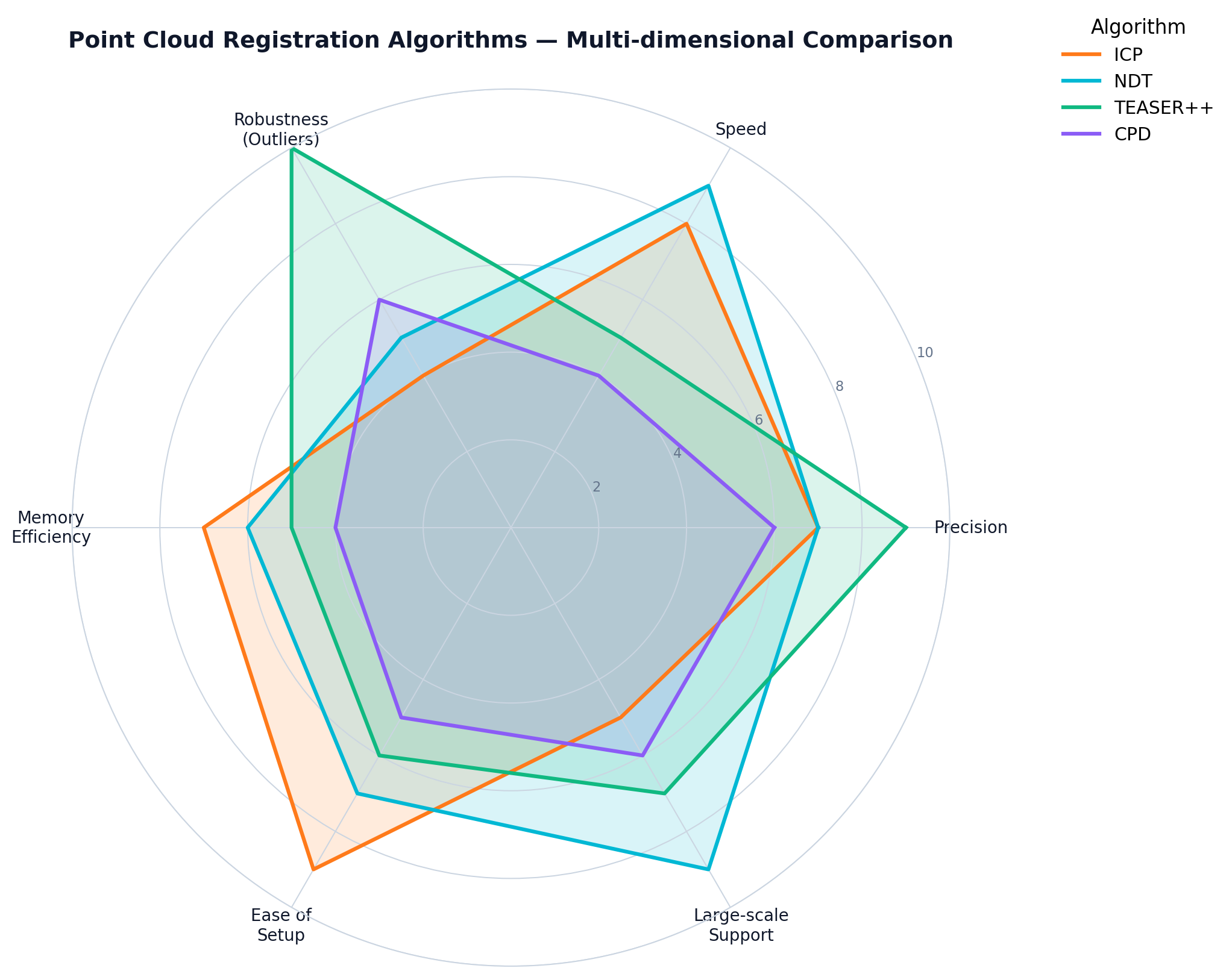
| Dimension | ICP | NDT | TEASER++ | CPD |
|---|---|---|---|---|
| Accuracy (clean data) | High | Medium-High | High | High |
| Accuracy (20%+ outliers) | Low | Low | High | Medium |
| Speed (10k points) | 5-15 ms | 2-5 ms | 30-80 ms | 50-150 ms |
| Speed (100k points) | 100-500 ms | 30-100 ms | 200-800 ms | >1 s |
| Outlier tolerance | Poor (needs filtering) | Poor (needs filtering) | Excellent (built-in) | Good (soft assignment) |
| Initial alignment need | Critical (local optima) | Moderate (multi-res helps) | Low (global-ish) | Moderate |
| Memory | O(n) for kd-tree | O(grid3) for grid | O(n) + SDP matrices | O(n×m) for correspondence |
| Non-rigid support | No | No | No | Yes |
| Best fit | Refinement, real-time | Large-scale SLAM | Coarse alignment, loop closure | Medical imaging, shape analysis |
A few takeaways from this table:
- ICP and NDT trade blows on clean data, but NDT wins on raw speed.
- TEASER++ is the only algorithm here that genuinely tolerates heavy outlier contamination without pre-filtering.
- CPD occupies a separate niche - if you need non-rigid alignment, nothing else in this list does it.
Where Each Algorithm Fits in Real Systems
Robotic Arm Grasping
Pick-and-place applications need millimeter-level accuracy on a known object. The sensor gives you a partial point cloud of the part, and you have a CAD model. ICP is the standard here: the CAD model provides a good initial alignment (from object detection), and ICP refines to sub-millimeter precision. GICP with point-to-plane error is the usual choice.
Mobile Robot SLAM
Autonomous mobile robots use LiDAR for localization and mapping. The sensor produces ~100k-300k points per scan at 10-20 Hz. Speed matters. Most production SLAM systems (Autoware, Apollo) use NDT or NDT variants for the scan-matching frontend because the speed advantage at high point counts is substantial.
For the loop closure problem - recognizing a previously visited location after a long trajectory - TEASER++ is increasingly popular. The point cloud difference at loop closure is typically large (different viewpoints, accumulated drift, missing/moved objects), so outlier tolerance matters more than speed.
3D Scanning and Reconstruction
Handheld and stationary 3D scanners capture overlapping point clouds from multiple viewpoints. The registration pipeline usually has two stages: coarse alignment (to bring overlapping scans within ICP's convergence basin), then fine alignment with ICP.
Feature-based methods (SAC-IA using FPFH descriptors, or Super4PCS using 4-point congruent sets) provide the coarse alignment, then ICP (often multi-scale) refines. The key requirement is sub-millimeter final accuracy for the refined model, which ICP delivers when given a reasonable starting point.
Indoor Mobile Mapping
Indoor mapping robots need to handle long corridors, rooms connected by doorways, and plenty of glass/mirror surfaces that produce ghost points. NDT works reasonably well for corridors (the planar structure fits the Gaussian assumption), but breaks down near corners and glass. ICP with aggressive outlier rejection (based on distance thresholds or normal compatibility) is more reliable in these environments.
Handheld Scanning
Handheld 3D scanners produce many overlapping frames with high overlap ratios (~60-80%) and small inter-frame motion. ICP performs well here because consecutive frames are naturally close in pose (handheld motion is smooth). Multi-scale ICP - coarse-to-fine correspondence distance - is the standard.
Choosing the Right Algorithm
There's no single best choice. The decision depends on data quality, computational budget, and downstream requirements.
Use ICP when: you have a decent initial alignment (from IMU, GPS, odometry, or object detection), your point clouds are relatively clean, and you need fast refinement. The workhorse that gets you 90% of the way in most robotics applications.
Use NDT when: speed is your primary constraint, you're working with large-scale outdoor point clouds, and you can tune the grid resolution for your environment. SLAM frontend on autonomous vehicles is the canonical use case. For 360° LiDARs with dense uniform point distribution, NDT grids fill more evenly - which is part of why NDT variants dominate outdoor SLAM.
Use TEASER++ when: your data is noisy, you have lots of outliers, or you need global-ish alignment without a good initial guess. It's slower, but it works when nothing else does. Common pattern: TEASER++ for coarse alignment, then ICP for refinement.
Use CPD when: you're dealing with deformable objects - medical imaging, shape analysis, character animation. Not a robotics algorithm, but worth knowing about if your work crosses into biomedical domains.
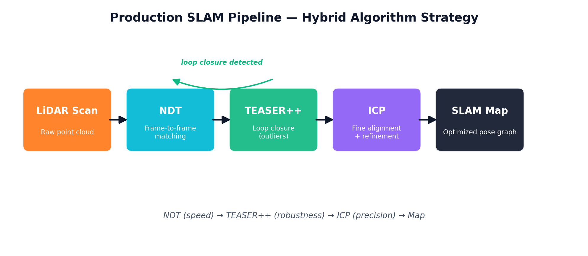
Use a combination: most production systems don't rely on a single method. A typical SLAM pipeline might use NDT for frame-to-frame matching, TEASER++ for loop closure candidates, and ICP for final sub-map refinement.
After registration, the next step in many LiDAR pipelines is annotation. For a comparison of annotation platforms, see our point cloud annotation tools comparison. For an inspection-focused workflow, see our LiDAR tunnel inspection guide.
Feature-based for coarse alignment: SAC-IA + FPFH or Super4PCS are alternatives when you have no prior pose estimate at all. They run slower than TEASER++ but don't require the SDP solver overhead.
Input Data Quality Matters More Than Algorithm Choice
This gets less attention than algorithm selection, but the quality of your input point clouds has a bigger impact on registration accuracy than which algorithm you pick.
Range accuracy determines how precisely each point represents the true surface. A LiDAR with ≤2 cm accuracy at 10 m gives your registration algorithm much less noise to deal with than a sensor with 5 cm accuracy. Angular resolution affects how well you capture edges and corners, which are the geometric features most registration algorithms depend on for finding correspondences. Point density matters too: sparse point clouds mean larger gaps in surface coverage, which makes nearest-neighbor matching less reliable.
Before optimizing your point cloud noise filtering pipeline, check what your sensor is actually putting out. A 360° LiDAR with ≤0.18° angular accuracy, ≤2 cm range precision, and 200 kHz point output rate provides high-quality input that lets every algorithm here work better. If you're evaluating hardware for a registration-heavy application, the full M360 specifications are worth a look.
If your registration results are inconsistent, check your sensor data before tuning algorithm parameters. A better point cloud makes every algorithm look good.
Comparing LiDAR sensors for your registration pipeline? See the M360 vs MID-360 comparison or contact our engineering team to discuss your specific requirements.