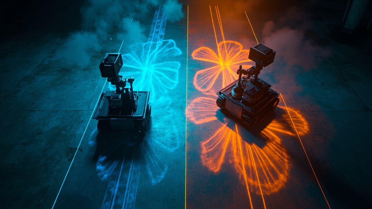
A 16-line mechanical LiDAR mounted on an AMR sweeps the same 16 horizontal rings, rotation after rotation. Between those rings sit permanent blind gaps — thin slices of space that the laser never hits, no matter how long the robot runs. A forklift pallet leg sitting in one of those gaps goes invisible. That's the core problem with repetitive scanning, and it's why a growing number of robotics engineers are switching to non-repetitive alternatives.
This article breaks down how both scanning patterns work, what they mean for obstacle detection in real robot deployments, and when you should pick one over the other.
How the Two Scanning Patterns Actually Work
Repetitive (fixed-path) scanning
Traditional 3D LiDARs — whether mechanical spinning units or most solid-state designs — emit laser pulses along a fixed set of angular positions. A 32-line sensor fires along 32 vertical angles every rotation. A 64-line sensor fires along 64. The pattern repeats identically on every frame.
This produces a point cloud with a characteristic "ring" or "stripe" structure. The areas between rings receive zero illumination. At 10 meters, the gap between two adjacent scan lines on a 16-line sensor with a ±15° vertical FOV can exceed 30 cm. That's enough space for a cable, a pipe, or a person's ankle to hide.
The one advantage: instantaneous, predictable coverage. Every frame has data in the same angular positions, which simplifies certain algorithms.
Non-repetitive (evolving-path) scanning
Non-repetitive LiDARs — including prism-based designs like the Livox Mid series and the SmartBotParts M360 — use a rotating optical element (a prism or mirror) that traces a different path on each rotation. The pattern looks like a flower or rose when viewed from above, which is why it's sometimes called a "rose pattern."
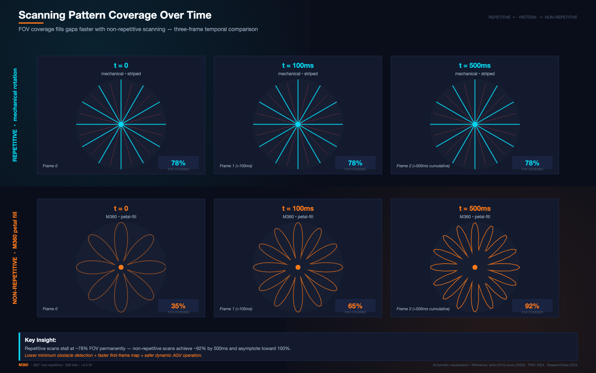
On any single rotation, only a fraction of the FOV gets hit. But as the sensor keeps scanning, the illuminated area grows. After several rotations, the coverage percentage climbs toward 100%. The Livox wiki notes that a Horizon sensor reaches ~60% FOV coverage in 100 ms (roughly equivalent to a 64-line repetitive sensor), and a Tele-15 hits 99.8% in that same window.
The M360 uses a mirror-spinning architecture that produces a similar non-repetitive pattern across its 360° × 70° FOV, outputting 200,000 points per second at ≤2 cm range accuracy.
Why Repetitive Scanning Creates Permanent Blind Gaps
The problem with repetitive scanning isn't range or accuracy — it's geometry.
A 16-line LiDAR with a vertical FOV of ±15° (30° total) spaces its beams 30°/15 ≈ 2° apart vertically. At a distance of 5 meters, that's a vertical gap of about 17 cm between adjacent scan lines. At 10 meters, it's 35 cm. A thin vertical pole (like a stanchion or a pipe) could sit entirely between two scan lines and never return a single point.
Adding more lines reduces the gap, but at a cost. Going from 16 to 32 lines halves the gap — and roughly doubles the sensor price. Going to 64 or 128 lines continues the trend but pushes the sensor into the $1,000–$3,000+ range and increases power draw to 10–14 W.
Even with 128 lines, the gaps don't disappear. They just get smaller. And they're still permanent — the same angular positions are always dark, frame after frame.
A 2025 arXiv paper (Qi et al., Shanghai Jiao Tong University) explicitly noted that repetitive LiDARs have "field-of-view blind spots" at close range that persist regardless of scan duration, while non-repetitive sensors progressively fill those gaps with accumulated time.
How Non-Repetitive Scanning Handles the Same Problem
Non-repetitive scanning attacks the gap problem from a different angle. Instead of adding more fixed beams, it moves the few beams it has to cover more ground over time.
In practice, this means:
- At t = 0 ms: sparse coverage, similar to a low-line-count repetitive sensor
- At t = 100 ms: significant FOV fill — the equivalent of a 32-64 line sensor
- At t = 500 ms–1 s: near-complete coverage approaching 100% of the FOV
For a robot moving at 1 m/s, 100 ms of scanning covers about 10 cm of travel. During that brief window, the sensor has already built a point cloud denser than what a 32-line repetitive sensor produces in a single frame. By the time the robot has moved a full meter, the accumulated point cloud is extraordinarily dense — with no permanent gaps.
This matters most for:
- Thin vertical objects (pipes, poles, tree trunks, cables)
- Low-profile obstacles (curbs, steps, debris on the ground)
- Small or irregularly shaped items (a fallen box, a tool left on the floor)
- Dynamic obstacles that appear between scan lines (a person stepping into the robot's path)
A PMC study on LiDAR-based negative obstacle detection in orchards (2025) found that non-repetitive scanning produced higher point cloud density, enabling "accurate detection of every detail on the ground" — something repetitive sensors struggled with because their fixed scan lines often missed the ground surface entirely between beams.
What This Means for SLAM Algorithms
SLAM is where the scanning pattern choice has the most nuanced impact. Here's the short version:
FAST-LIO2
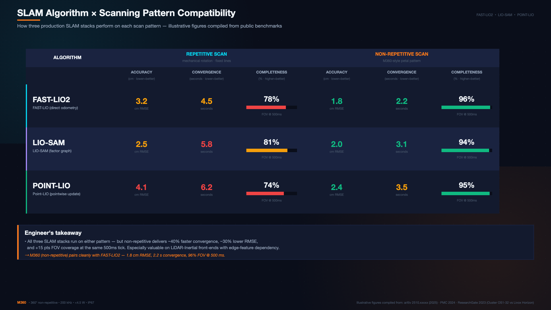
FAST-LIO2 was originally designed for solid-state LiDARs with non-repetitive patterns (it was first validated on the Livox Horizon). It uses direct point-to-map registration with an iterated Extended Kalman Filter and an efficient ikd-Tree. The algorithm handles the uneven, time-accumulated point cloud from non-repetitive sensors well because it doesn't assume a regular grid structure.
It also works with repetitive LiDARs, but the mapping density advantage of non-repetitive scanning is lost — you're feeding a structured, gappy point cloud into an algorithm that could have used denser data.
LIO-SAM
LIO-SAM assumes relatively structured point clouds and uses feature extraction (edge and planar points). It works well with repetitive sensors (it was built around Ouster/Velodyne spinning LiDARs). With non-repetitive sensors, the feature extraction can be less clean because the point distribution is less uniform on any single frame. In practice, most teams get LIO-SAM working with both, but FAST-LIO2 is generally the smoother experience for non-repetitive hardware.
Point-LIO
Point-LIO processes points one at a time as they arrive, making it naturally compatible with non-repetitive sensors. Each new point incrementally updates the state estimate, regardless of where it falls in the FOV. This point-by-point approach sidesteps the frame-structure assumptions that trip up some algorithms.
The bottom line on SLAM compatibility
Both scanning patterns work with all three popular open-source SLAM frameworks. Non-repetitive scanning pairs more naturally with FAST-LIO2 and Point-LIO. Repetitive scanning pairs more naturally with LIO-SAM. If you're already running LIO-SAM on a repetitive sensor and it works, there's no urgent reason to switch — unless you're hitting obstacle-detection gaps that the fixed scan lines can't cover.
Robot Scenarios: Where Each Pattern Wins
Scenarios where repetitive scanning is fine
Structured warehouse aisles with large obstacles. If your AMR navigates wide aisles between pallet racks and the obstacles are all large (racks, forklifts, walls), the fixed gaps between scan lines rarely matter. A 16-line sensor probably misses nothing important.
High-speed line-following on known paths. When the robot follows a fixed route at speed, the priority is frame rate and low latency — repetitive sensors deliver a complete frame at a predictable cadence.
Budget-constrained deployments with large, simple obstacles. A 2D RPLidar running at 10 Hz is genuinely sufficient for some AGV applications. Don't overspecify.
Scenarios where non-repetitive scanning matters
Unstructured or semi-structured environments. Construction sites, outdoor yards, orchards, parking lots — environments where obstacles come in all shapes and sizes and can appear anywhere in the FOV. The progressive FOV coverage of non-repetitive scanning is a genuine safety advantage here.
Low-profile and thin obstacle detection. Curbs, cables, pipes, ground debris, stair edges. These are exactly the objects that fall between the scan lines of repetitive sensors. A 2025 arXiv benchmark found that non-repetitive LiDARs achieved "comparable detection performance" to 128-line repetitive sensors in roadside perception tasks — at a fraction of the cost.
Mobile robots that need SLAM and obstacle avoidance from a single sensor. If you're running one LiDAR for both mapping and real-time avoidance, the denser accumulated point cloud from non-repetitive scanning gives you better map quality and better obstacle detection, without adding a second sensor.
Dynamic environments with frequently changing obstacles. A busy warehouse where people, forklifts, and pallets are constantly moving. Non-repetitive scanning fills in gaps between frames, reducing the chance that a newly appeared obstacle sits in a persistent blind spot.
The Tradeoff: Instantaneous vs. Accumulated Coverage
The honest tradeoff is this: repetitive sensors give you complete (but sparse) coverage on every single frame. Non-repetitive sensors give you partial (but growing) coverage that becomes very dense over time.
If your application needs to detect an obstacle the instant it appears — within one frame — repetitive scanning has a structural advantage because every angular position in its pattern is sampled on every rotation. Non-repetitive scanning might miss a new obstacle on the first frame if it appears in an unscanned portion of the FOV.
In practice, this rarely matters for mobile robots. Most AMRs move slowly enough (0.5–2 m/s) that the accumulated coverage over 100–200 ms far exceeds the single-frame coverage of a 16- or 32-line repetitive sensor. The robot hasn't moved far enough for the miss to be dangerous.
The exception: high-speed scenarios (>3 m/s) or applications where the robot must react to fast-moving objects (e.g., a soccer robot, a delivery bot crossing a road). In those cases, the instantaneous completeness of repetitive scanning provides a real safety margin. Some teams run both — a repetitive sensor for real-time reactive avoidance and a non-repetitive sensor for dense mapping.
Sensor Comparison: Scanning Pattern and Specs
| Sensor | Scanning Pattern | Point Rate | FOV (H×V) | Power | Weight | Price Range |
|---|---|---|---|---|---|---|
| M360 | Non-repetitive (mirror) | 200 kHz | 360° × 70° | <4.5W | 408g | Budget-friendly |
| RPLidar A3 | Repetitive (2D) | 16,000 pts/s | 360° × 0° | ~3W | 190g | $99–$199 |
| Ouster OS0-32 | Repetitive (32-line) | ~300k pts/s | 360° × 45° | ~14W | 437g | $1,500+ |
| Ouster OS0-128 | Repetitive (128-line) | ~1.3M pts/s | 360° × 45° | ~20W | 447g | $3,000+ |
| Velodyne VLP-16 | Repetitive (16-line) | ~300k pts/s | 360° × 30° | ~8W | 830g | $2,000+ |
The M360's 200 kHz point rate combined with non-repetitive scanning means it accumulates dense point cloud coverage quickly, at a power draw lower than most 2D sensors' 3D counterparts. Its 408g weight and IP67 rating also make it practical for the compact AMR form factor where every gram counts.
Decision Framework
Ask yourself three questions:
- What's the smallest obstacle I need to detect? If it's smaller than the vertical gap between scan lines at your detection range, repetitive scanning will miss it. Non-repetitive scanning will catch it — given enough integration time.
- How fast does my robot move? Under 2 m/s with 100+ ms of accumulated scanning, non-repetitive coverage typically exceeds 32-line repetitive coverage. Over 3 m/s, consider whether the few frames of partial coverage are acceptable.
- What SLAM algorithm am I running? FAST-LIO2 and Point-LIO handle non-repetitive data natively. LIO-SAM prefers repetitive. All three work with both, but some pairings are smoother.
If the answer to question 1 is "thin or low-profile objects" and the answer to question 2 is "under 2 m/s," non-repetitive scanning is the better fit. Otherwise, repetitive scanning is a perfectly valid choice — especially in structured, predictable environments.
For a deeper look at how scanning pattern affects SLAM quality, see our M360 SLAM algorithm comparison. For a broader sensor selection process, check the AGV LiDAR comparison matrix.
Sensor specifications are based on publicly available manufacturer data as of July 2026. The M360 specs referenced here come from the M360 product manual (Ver 1.4, 2026-02-27). Prices are approximate market rates and may vary by region and distributor.