Selecting a LiDAR sensor for automated guided vehicles feels straightforward on paper. You pull up a few datasheets, compare detection range, field of view, and price tag, and pick the one that looks best. In practice, that approach lands teams in trouble more often than not.
Over the past three years, we have reviewed deployment data from warehouse operations, manufacturing plants, and port logistics hubs across North America and Europe. The pattern that keeps showing up is consistent: roughly 60% of AGV fleet operators who selected their LiDAR based on spec-sheet comparisons alone ran into problems within the first 18 months. Those problems ranged from integration headaches to unexpected downtime and costs that dwarfed the original hardware purchase.
This guide walks through the evaluation methodology that separates a sound sensor choice from an expensive mistake. The sections below cover the eight hardware parameters that actually matter, the software compatibility factors most teams overlook, a total cost of ownership model with estimated numbers, and a 15-point checklist you can put to work right away.
For a comprehensive overview of LiDAR types and use cases, see our AGV/AMR LiDAR selection guide.
8 Hardware Parameters for AGV LiDAR Selection
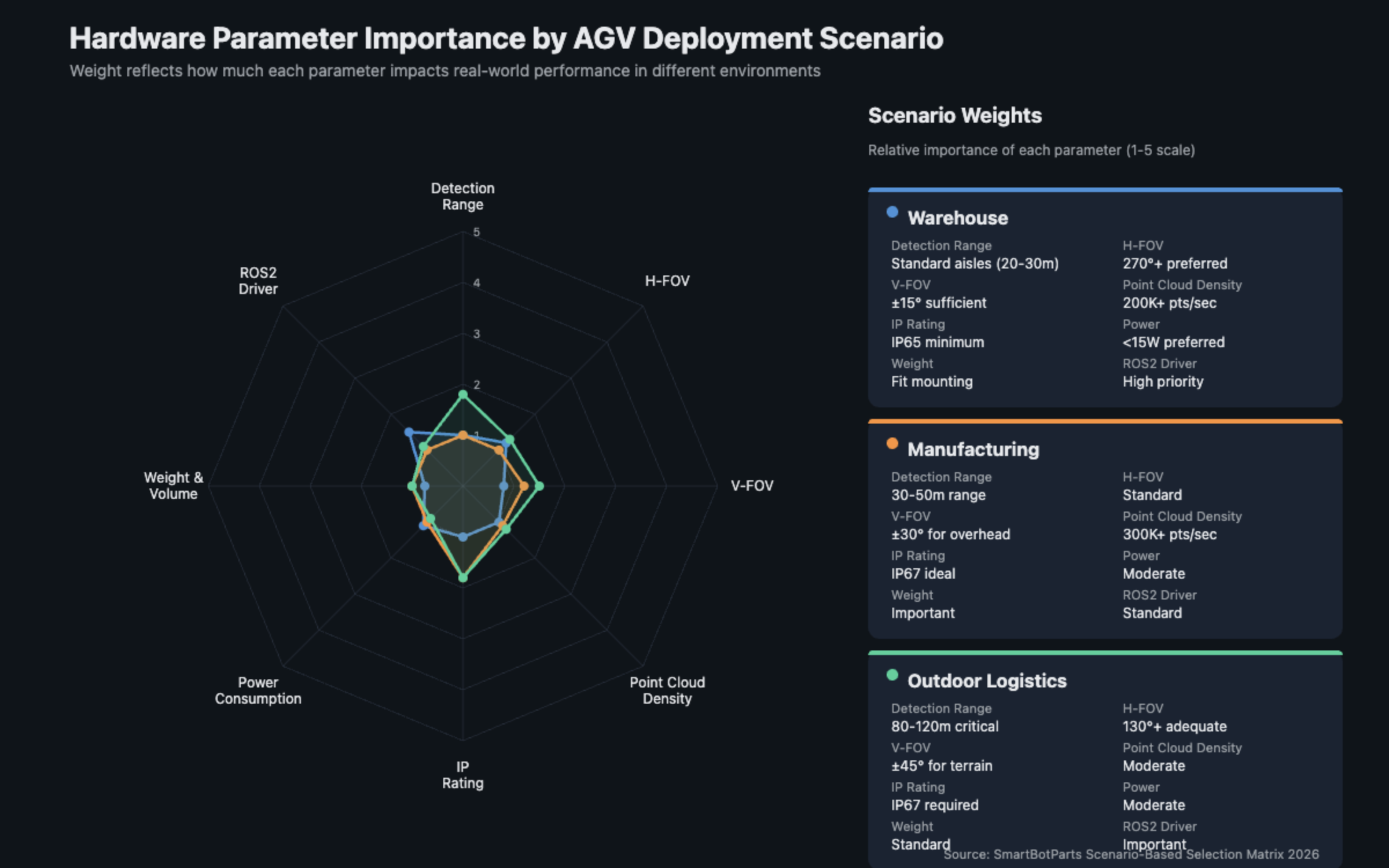
Most LiDAR datasheets list 15 to 20 specifications. The majority of those numbers are noise for AGV applications. Here are the eight that drive real-world performance differences.
Detection Range: Match It to Your Environment, Not Your Ego
LiDAR detection range is the single most overspecified parameter in AGV fleet procurement. A 200-meter detection range catches the eye on a comparison chart, but if your longest aisle measures 40 meters, you are paying for range you will never use. In some designs, that extra range comes at the cost of refresh rate or angular resolution.
The practical approach is to calculate your maximum required detection distance and add a 20% safety margin. For most indoor warehouse AGVs operating in standard rack aisles (typically 8-12 meters wide), a detection range of 20-30 meters is sufficient. Manufacturing AGVs navigating between production lines might need 30-50 meters. Outdoor logistics vehicles handling container yards can justify 80-120 meters.
Overspecifying range carries a hidden penalty. Longer-range LiDAR units typically consume more power, generate more heat, and cost more. When you are deploying 50 or 100 units, that per-unit cost difference compounds fast. One fleet operator we surveyed specified 100-meter sensors for indoor warehouse AGVs running 25-meter routes. They spent 40% more on hardware than necessary and saw no performance improvement over the 30-meter units their original proposal had included.
For a detailed look at how near-blind zones affect detection accuracy, see our AGV LiDAR blind zone comparison (6 sensors).
Field of View: Horizontal and Vertical Coverage Trade-Offs
Field of view determines how much of the surrounding environment a single LiDAR can monitor without mechanical scanning. For AGV LiDAR selection, the horizontal FOV gets most of the attention, but the vertical FOV is often more important than people realize.
Indoor warehouse AGVs generally operate in environments where obstacles appear at ground level: pallets, forklift tines, shrink-wrapped loads. A vertical FOV of ±15° is usually enough for these applications. Manufacturing environments with overhead obstacles, conveyor belts, and multi-level racking benefit from ±30° or wider vertical coverage. Outdoor applications dealing with uneven terrain, loading ramps, and varying vehicle heights push the requirement to ±45° or more.
Here is where the field of view calculation gets interesting from a cost perspective. A single 3D LiDAR with 360° horizontal and wide vertical FOV might cost $2,500-$4,000. A pair of 2D LiDAR units (one front-mounted, one rear-mounted) could cover the same horizontal arc for $600-$1,200 total. The trade-off is vertical coverage and point cloud density, which matters in complex environments. For simple point-to-point transport routes, the two-sensor approach is often the better deal.
Another option worth evaluating: a single 2D LiDAR with a small servo or rotating mount for vertical scanning. This adds mechanical complexity but can achieve selective vertical coverage at a fraction of the cost of a full 3D unit. Several logistics operators in Europe have adopted this approach for narrow-aisle warehouse AGVs with solid results.
Point Cloud Density vs. Processing Overhead
Point cloud density, measured in points per second, determines how well your AGV can distinguish between objects. A human leg, a pallet corner, and a cable on the floor all look different when you have enough points hitting them. With sparse point clouds, they blur together, and your obstacle detection accuracy drops.
The catch is that higher point density demands more processing power on your onboard computer. At 300,000 points per second, a standard industrial PC handles SLAM and obstacle detection comfortably. Push that to 1.2 million points per second, and you might need a more expensive compute platform or risk increased latency in your safety-critical detection loop.
The right density depends on what you need to detect. Simple navigation along fixed paths with large, obvious obstacles (full pallets, vehicles) can work fine at 100,000-200,000 points per second. Environments with small obstacles (cables, dropped tools, low-profile items on the floor) benefit from 300,000-600,000 points per second. High-precision manufacturing or sorting applications may justify 600,000+ points per second.
IP Rating: IP65 Is Not the Same as IP67
The IP (Ingress Protection) rating is one of those specifications that teams often treat as a checkbox item. It should not be. The difference between IP65 and IP67 is the difference between a sensor that survives a wet warehouse floor and one that does not.
IP65 protects against dust ingress and low-pressure water jets from any direction. IP67 adds temporary immersion protection: the sensor can survive being submerged in up to 1 meter of water for 30 minutes. In practice, this matters for cold storage facilities where condensation and ice buildup are constant, washdown areas in food processing, and outdoor logistics operations that encounter heavy rain or flooding.
The cost premium for IP67 over IP65 varies by manufacturer but typically runs 15-30%. For indoor dry environments, IP65 is almost always sufficient. If your AGVs operate in cold storage, food processing, or outdoor settings, the IP67 upgrade pays for itself quickly by preventing water-damage failures.
Power Consumption: It Adds Up Across a Fleet
LiDAR power consumption rarely makes or breaks a single-unit decision. Across a fleet of 50 or more AGVs running 24/7, it becomes a real operational expense that teams often forget to budget for.
A low-power 2D LiDAR might draw 3-5 watts. A mid-range 3D unit typically consumes 10-15 watts. High-performance sensors can pull 20-30 watts or more. Across a 50-unit fleet running continuously, the difference between 5 watts and 25 watts per unit is 1,000 watts, roughly the power consumption of a small office, running 24 hours a day, 365 days a year.
At an industrial electricity rate of $0.08 per kWh, that difference works out to roughly $700 per year in additional power costs for the fleet. Not a deal-breaker, but not negligible either, especially when you add cooling requirements. Higher-power sensors generate more heat, which means your AGV's onboard cooling system works harder, shortens fan lifespan, and may require more frequent maintenance.
Weight and Volume: The Payload Penalty
Every gram counts on an AGV. The sensor weight directly reduces the vehicle's usable payload capacity. A 2D LiDAR weighing 130 grams barely registers. A 3D LiDAR weighing 800 grams takes a noticeable bite out of your payload budget.
For a small warehouse AGV with a 50 kg payload capacity, adding an 800-gram sensor reduces usable payload by 1.6%. That sounds small, but if you are already near the limit with a loaded pallet, it can mean one fewer items per trip, which translates to more trips per shift, which translates to more wear on the vehicle and higher operating costs.
The volume consideration matters for AGVs with tight mounting constraints. Some 3D LiDAR units are compact enough to mount inside the vehicle body. Others require external mounting brackets that increase the vehicle's physical footprint. That is a problem in narrow aisle operations where every centimeter of clearance matters.
Interface and Protocol: Integration Ease
The physical and data interface of your LiDAR determines how much engineering effort your integration team will spend. The main options break down as follows:
- Ethernet (100M/1G): Most common for 3D LiDAR. High bandwidth, supports dense point clouds, but requires an Ethernet switch or hub on the AGV and cable routing. Integration complexity is moderate.
- CAN Bus: Common in automotive-grade sensors and well-suited to noisy industrial environments. Bandwidth is limited, which restricts point cloud density. Integration is straightforward if your AGV already runs a CAN-based architecture.
- UART/Serial: Found on budget 2D LiDAR units. Low bandwidth, suitable only for simple point cloud data. Easy to integrate but limits future expandability.
The practical advice: pick a LiDAR with an interface that matches your AGV's existing data architecture. Adding an Ethernet switch and routing Cat6 cable through a vehicle that was designed around CAN bus is not a trivial engineering task. One systems integrator reported spending 120 additional engineering hours per vehicle to retrofit Ethernet connectivity for a sensor that only shipped with Ethernet, when the AGV's control architecture was CAN-based. At $150 per hour, that is $18,000 in unplanned integration cost per vehicle.
Operating Temperature Range: Cold and Heat Degrade Performance Differently
LiDAR operating temperature specifications are often misleading because they tell you the survival range, not the performance range. A sensor rated for -20°C to +55°C might survive at those extremes, but its detection accuracy and point cloud quality can degrade significantly at the edges.
In cold environments, laser diode output drops, which reduces detection range. One cold-chain operator reported a 15% range reduction at -20°C compared to room-temperature specs for their mid-range 3D LiDAR. In hot environments, thermal noise increases, which degrades point cloud quality. The degradation curve is rarely linear, and most manufacturers do not publish it. If the vendor cannot provide temperature-specific performance data, request a loan unit for testing in your actual operating conditions.
For cold storage operations (-25°C to +5°C), ask manufacturers for cold-temperature performance data, not just survival specifications. For outdoor applications in hot climates (40°C+ ambient), ask about derating curves and whether active cooling is required to maintain rated performance.
LiDAR Software Ecosystem: Why It Matters More Than Hardware Specs
A LiDAR sensor without solid software support becomes an expensive paperweight. The software stack around the sensor determines how quickly you can integrate it, how well it performs with your existing navigation stack, and how much ongoing maintenance your engineering team will need to provide. We have seen procurement decisions stall for months because a hardware team selected a sensor whose software support could not meet the integration timeline.
ROS and ROS2 Driver Support
The Robot Operating System has become the de facto standard for AGV navigation. A LiDAR with official, well-maintained ROS2 drivers saves weeks of integration work. A LiDAR with only proprietary SDKs or unmaintained community drivers costs you engineering time.
Check the driver repository for the sensor you are evaluating. Look at the commit history. Is it actively maintained? Check the issues list. Are there unresolved problems that affect AGV use cases? A driver that has not seen a commit in 12 months is a red flag.
Some manufacturers maintain their drivers in-house and release them through their own repositories. Others rely on community-maintained drivers. In-house maintenance provides better accountability, but community drivers can offer faster bug fixes and wider testing across different use cases.
SDK Quality and Documentation
The SDK quality affects everything from initial integration to ongoing debugging. A good SDK provides clean APIs with clear documentation, working example code, and responsive technical support. A poor SDK means your engineers spend days reverse-engineering data formats and debugging undocumented behavior.
When evaluating SDK quality, look for three things: API documentation completeness (are all data fields documented, or are some marked "internal"?), example code quality (does the manufacturer provide working examples for common AGV tasks like obstacle detection and SLAM?), and community activity (are other developers using this SDK and discussing it in forums?).
SLAM Algorithm Compatibility
Your LiDAR's point cloud format needs to work with your SLAM algorithm. The most common open-source SLAM solutions for AGV applications, including FAST-LIO2, LIO-SAM, and Cartographer, have different input requirements and optimization profiles.
FAST-LIO2, for example, is designed for solid-state LiDAR with non-repetitive scanning patterns and works best with point clouds at specific rates. LIO-SAM requires IMU data fused with LiDAR for best results. Cartographer is more forgiving but computationally heavier.
The practical test: before committing to a LiDAR purchase, run your target SLAM algorithm with sample data from that sensor. Most manufacturers can provide sample point cloud datasets. This 30-minute test can save you weeks of integration headaches. If the manufacturer cannot provide sample data, that is itself a signal about their software maturity and customer support readiness.
For product-specific SLAM compatibility data, see our best 3D LiDAR for robot SLAM (2025 comparison).
PTP Time Synchronization for Multi-LiDAR Deployments
If your AGV uses more than one LiDAR sensor, precise time synchronization between the sensors is not optional. Without synchronized timestamps, your point clouds from different sensors cannot be accurately aligned, and your perception pipeline produces ghost artifacts and inconsistent obstacle detection.
IEEE 1588 Precision Time Protocol (PTP) support is the gold standard for multi-LiDAR synchronization. Sensors without PTP support require software-based synchronization, which introduces jitter and reduces alignment accuracy. For multi-sensor AGVs operating in environments with tight clearance requirements, PTP is worth the additional sensor cost. Ask your sensor vendor whether their PTP implementation supports the AGV's real-time operating system. Not all PTP stacks play nicely with all RTOS platforms.
The Hidden Costs No Datasheet Tells You: A TCO Analysis
Hardware purchase price is the most visible cost of a LiDAR deployment. It is also the smallest cost for most fleets running three years or more. The total cost of ownership includes six major cost categories that most selection frameworks ignore.
The Six Components of LiDAR TCO
- Hardware purchase price: The upfront cost per unit, multiplied by fleet size.
- Calibration and maintenance labor: External calibration frequency (typically quarterly for 3D LiDAR), time per calibration, and technician hourly rate.
- Spare parts inventory: Critical spare parts held on-site, including replacement cost and holding cost.
- Downtime cost from failures: Revenue lost per hour of vehicle downtime, multiplied by estimated annual failure hours.
- Software licensing: SLAM algorithm licenses, point cloud processing software, and driver maintenance contracts.
- Training and onboarding: Engineering hours spent learning the sensor platform and training maintenance staff.
3-Year TCO Model: By Price Tier
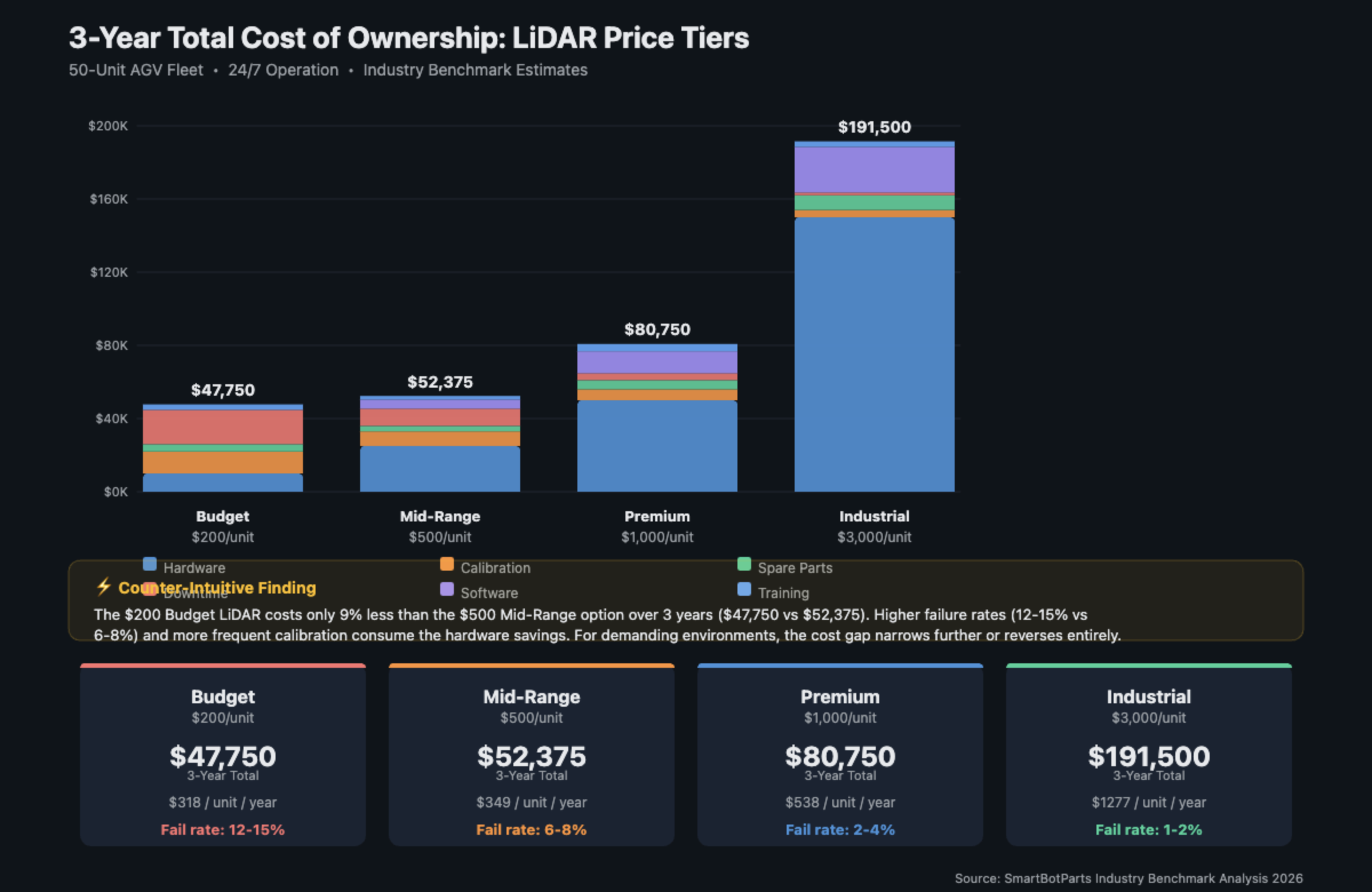
The table below presents a 3-year TCO comparison across four LiDAR price tiers for a 50-unit AGV fleet running 24/7. All figures are estimated based on industry benchmarks and publicly available data from fleet operators. For a deeper dive, see our full TCO analysis article.
| Cost Category | Budget Tier ($200/unit) | Mid-Range ($500/unit) | Premium ($1,000/unit) | Industrial ($3,000/unit) |
|---|---|---|---|---|
| Hardware (50 units) | $10,000 | $25,000 | $50,000 | $150,000 |
| Calibration labor (4x/yr, 2hr each) | $12,000 | $8,000 | $6,000 | $4,000 |
| Spare parts (held on-site) | $4,000 | $3,000 | $5,000 | $8,000 |
| Failure downtime (est. annual hrs) | $18,750 (150 hrs @ $125/hr) | $9,375 (75 hrs) | $3,750 (30 hrs) | $1,500 (12 hrs) |
| Software licensing | $0 (open source only) | $5,000 | $12,000 | $25,000 |
| Training (initial + ongoing) | $3,000 | $2,000 | $4,000 | $3,000 |
| 3-Year TCO | $47,750 | $52,375 | $80,750 | $191,500 |
| TCO per unit, per year | $318 | $349 | $538 | $1,277 |
| Annual failure rate (est.) | 12-15% | 6-8% | 2-4% | 1-2% |
A few observations from this model that surprise people:
The budget $200 LiDAR does not actually save money over three years compared to the mid-range $500 option. Higher failure rates and more frequent calibration requirements eat into the hardware savings. If your AGVs operate in demanding environments (dust, vibration, temperature cycling), the gap widens further because budget sensors degrade faster under stress.
The premium $1,000 tier starts to show its value when you factor in reduced downtime. For operations where vehicle downtime costs exceed $125 per hour, the reliability improvement pays for the hardware premium within 18 months.
The industrial $3,000 tier is hard to justify purely on TCO for standard warehouse applications. It makes sense for harsh environments (ports, cold storage, chemical plants) where the sensor's durability prevents failures that would cost more in downtime and safety incidents.
When considering alternatives at each tier, check out our 7 alternatives to Livox Mid-360 for brand-specific cost comparisons.
Calibration: The Cost Nobody Budgets For
External calibration, the process of aligning the LiDAR's coordinate frame to the vehicle's chassis, is required after initial installation and on an ongoing basis. Vibration, thermal cycling, and physical impacts all cause calibration drift.
Budget 2D LiDAR units typically need recalibration every 2-3 months because they use lower-grade mounting hardware and have less stable optical assemblies. Premium 3D LiDAR units can often go 6-12 months between calibrations. The difference is not just the labor cost. It is the vehicle downtime during calibration, which for a busy warehouse can represent real revenue loss.
One cold storage operator shared their calibration logs with us: their budget 2D sensors required recalibration every 6 weeks because thermal cycling caused the mounting brackets to shift. Each recalibration took 90 minutes per vehicle plus 30 minutes of cooldown before the vehicle could return to service. With 20 vehicles in the fleet, that was 40 hours of vehicle downtime per calibration cycle. At their throughput rate, each hour of downtime cost approximately $180 in delayed order fulfillment.
2D vs. 3D: When the Upgrade Actually Pays Off
The question of whether to upgrade from 2D to 3D LiDAR comes up in almost every AGV fleet planning discussion. The answer depends on your environment, not on marketing claims. For a comprehensive upgrade analysis, see our 2D vs 3D LiDAR upgrade analysis.
Where 2D LiDAR Still Works
2D LiDAR remains the right choice for several common AGV scenarios:
- Fixed-path transport in clean, controlled warehouse environments with well-defined corridors.
- Simple obstacle detection where all obstacles are tall enough to intersect the laser plane (full pallets, walls, vehicles).
- Fleet sizes over 100 units where the per-unit cost difference between 2D and 3D makes a meaningful impact on the total budget.
- Battery-constrained vehicles where the 5-15 watt power savings of 2D LiDAR extends operating time per charge.
The Value Inflection Point for 3D
3D LiDAR starts delivering returns in environments where 2D falls short:
- Dynamic environments with obstacles at varying heights: forklifts, overhead conveyors, multi-level storage, and partially loaded pallets.
- Mixed-traffic areas where pedestrians share space with AGVs and height-based classification (telling a person from a pallet) reduces false emergency stops.
- Unstructured outdoor areas with uneven surfaces, loading ramps, and obstacles that a single horizontal scan plane would miss entirely.
- High-value payload operations where collision avoidance accuracy directly prevents expensive product damage and insurance claims.
ROI Calculation: 2D to 3D Upgrade
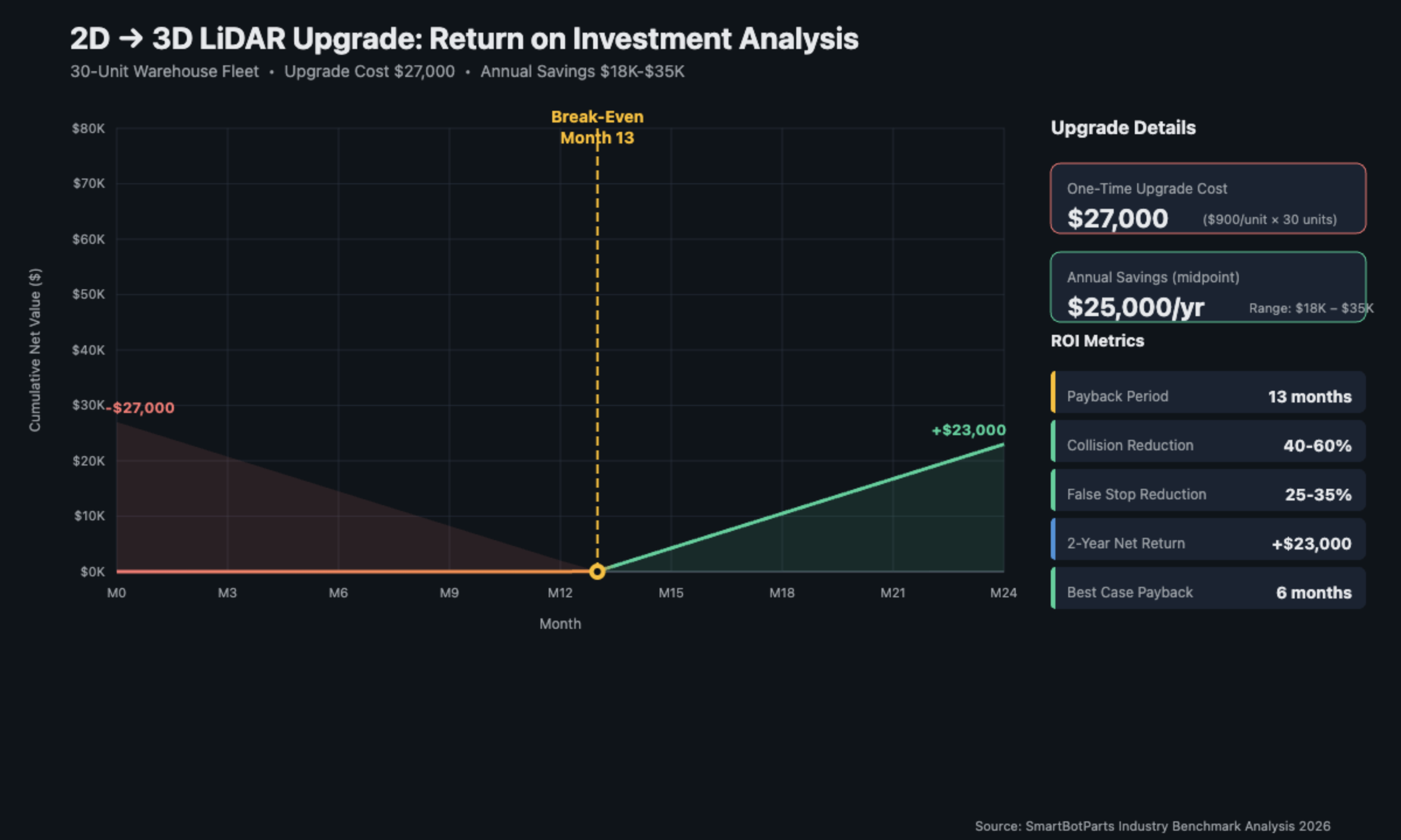
Consider a 30-unit warehouse fleet currently running 2D LiDAR. The upgrade cost to 3D is approximately $900 per unit ($1,000 sensor minus $100 credit for the existing 2D unit), totaling $27,000.
Based on operator-reported data from similar upgrades:
- Collision rate reduction: 40-60% (3D detects low-profile and overhead obstacles that 2D misses).
- False-positive emergency stops reduction: 25-35% (3D point clouds provide better object classification, reducing unnecessary stops).
- Annual savings from reduced collisions and stops: $18,000-$35,000 (varies by payload value and throughput requirements).
At the midpoint estimate of $25,000 in annual savings, the upgrade pays for itself in roughly 13 months. For fleets carrying high-value goods or operating at near-maximum throughput, the payback period can be under 8 months. One automotive parts distributor reported that upgrading their 40-vehicle fleet from 2D to 3D LiDAR eliminated an average of 3 collision incidents per month, each costing $2,000 to $5,000 in damaged product and vehicle repair. Their upgrade paid for itself in under 6 months.
For 3D LiDAR options that offer strong ROI, consider the M360 3D LiDAR sensor.
Multi-LiDAR Deployment Considerations
As AGVs get more capable and environments get more complex, fleets are moving from single-sensor to multi-sensor configurations. This introduces a new layer of cost and complexity that most teams underestimate.
Cross-sensor interference occurs when two or more LiDAR units on the same vehicle detect each other's laser pulses, creating ghost points in the point cloud. Most modern sensors include some form of interference mitigation, but the effectiveness varies widely. Budget sensors often rely on simple temporal filtering that reduces the problem but does not eliminate it. Premium sensors use more sophisticated approaches like random pulse timing or wavelength separation.
The practical impact: if your AGV uses three LiDAR units (front, rear, and top-mounted), sensor interference adds noise to your point cloud that your perception algorithm must filter out. More noise means higher computational requirements for your obstacle detection, which can push you toward a more expensive onboard computer. The problem of a "cheap sensor that needs a $500 compute upgrade" shows up regularly in fleet deployments.
Configuration management is another underestimated cost. Each LiDAR in a multi-sensor setup needs its own calibration, its own driver configuration, and its own health monitoring. For a 50-vehicle fleet with 3 sensors per vehicle, that is 150 sensor configurations to maintain, calibrate, and monitor across the fleet lifecycle.
AGV LiDAR Selection Matrix: 5 Scenario-Based Frameworks
Rather than recommending specific brands, here is a weighted scoring framework you can apply to any LiDAR product for your specific deployment scenario. Rate each parameter on a 1-5 scale (5 = excellent for your use case) and multiply by the weight.
Warehouse AGV (Indoor, Standard Environment)
| Parameter | Weight | Your Rating | Weighted Score |
|---|---|---|---|
| Detection range (20-30m sufficient) | 1.0 | ___ | ___ |
| Horizontal FOV (270°+ preferred) | 1.2 | ___ | ___ |
| Vertical FOV (±15° typically sufficient) | 0.8 | ___ | ___ |
| Point cloud density (200K+ pts/sec) | 1.0 | ___ | ___ |
| IP rating (IP65 minimum) | 1.0 | ___ | ___ |
| Power consumption (<15W preferred) | 1.1 | ___ | ___ |
| ROS2 driver quality | 1.5 | ___ | ___ |
| SLAM compatibility | 1.5 | ___ | ___ |
| 3-year TCO per unit | 1.3 | ___ | ___ |
| Annual failure rate | 1.2 | ___ | ___ |
| Total weighted score | ___ / 70 |
A score above 50 indicates a strong fit for standard warehouse AGV use.
Manufacturing AGV (Dust, Vibration, Temperature Extremes)
Same parameters, but adjust the weights: IP rating (1.8), operating temperature range (1.5), vibration tolerance (1.5), annual failure rate (1.5), and reduce SLAM compatibility weight (1.0) since manufacturing paths are often more structured.
Outdoor Logistics AGV (Weather, Variable Lighting)
Adjust weights: detection range (1.8), IP67 rating (1.8), operating temperature range (1.5), horizontal FOV (1.3), sunlight immunity (1.5), and PTP synchronization (1.3 if multi-sensor).
Port and Container AGV (Extreme Environment, Long Range)
Adjust weights: detection range (2.0), IP67 or higher (2.0), vibration tolerance (1.8), operating temperature range (1.5), annual failure rate (1.8), and TCO per unit (1.5).
Cold Storage AGV (Low Temperature, High Humidity)
Adjust weights: IP67 with condensation resistance (2.0), cold-temperature performance (2.0), defrost/anti-ice capability (1.8), power consumption (1.5, less waste heat to manage), and annual failure rate (1.5).
The 15-Point LiDAR Evaluation Checklist
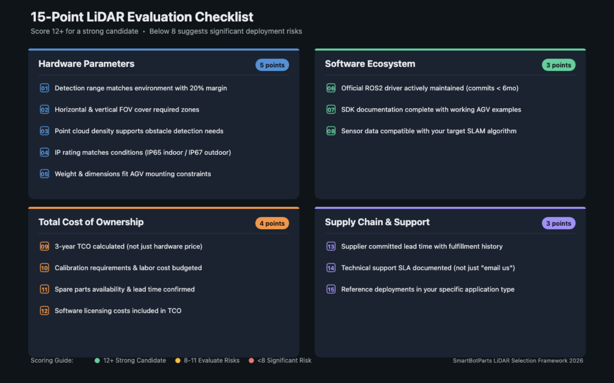
Print this checklist. Fill it out for every LiDAR you shortlist. A sensor that scores 12 or above across all categories is a strong candidate. Anything below 8 suggests significant risks for your deployment.
Hardware Parameters (5 points)
- 1. Detection range matches environment with 20% margin (no significant overspec)
- 2. Horizontal and vertical FOV cover required monitoring zones
- 3. Point cloud density supports required obstacle detection granularity
- 4. IP rating matches environmental conditions (IP65 indoor, IP67 outdoor/wet)
- 5. Weight and dimensions fit AGV mounting constraints without payload penalty
Software Ecosystem (3 points)
- 6. Official ROS2 driver is actively maintained (commits within 6 months)
- 7. SDK documentation is complete with working AGV-relevant example code
- 8. Sensor data format is confirmed compatible with your target SLAM algorithm
Total Cost of Ownership (4 points)
- 9. 3-year TCO has been calculated (not just hardware price)
- 10. Annual calibration requirements and labor cost are known and budgeted
- 11. Spare parts availability and lead time confirmed with the supplier
- 12. Software licensing costs (SLAM, processing tools) are included in TCO
Supply Chain and Support (3 points)
- 13. Supplier provides committed lead time with trackable fulfillment history
- 14. Technical support response SLA is documented (not just "email us")
- 15. Reference deployments exist in your specific application type (not just "industrial use")
Where to Go From Here
The LiDAR market for AGV applications has more options than ever, and the range of quality and reliability across those options is wide. The sensors that look best on a spec sheet are not always the ones that deliver the lowest total cost over three years of fleet operation.
The framework laid out in this article, covering eight hardware parameters, software compatibility evaluation, TCO modeling, and the 15-point checklist, gives you a repeatable process for making that decision with data instead of guesswork.
If you want help applying this framework to your specific fleet requirements, SmartBotParts offers a no-cost consultation that walks through the scoring matrix with your actual operating parameters. No hard sell, no brand pushing. Just an honest technical assessment of which LiDAR characteristics matter most for your deployment, and a shortlist that fits your budget and environment. You can reach the team through the contact form on the SmartBotParts website.
For a printable version of the 15-point checklist to use with your procurement team, download the PDF version here. For additional procurement guidance, see our practical checklist for after buying 20+ LiDARs.
Frequently Asked Questions
How do I choose the right detection range for AGV LiDAR?
Calculate your maximum required detection distance and add a 20% safety margin. For indoor warehouse AGVs in standard rack aisles (8-12m wide), 20-30 meters is sufficient. Manufacturing AGVs between production lines need 30-50 meters. Outdoor logistics vehicles handling container yards can justify 80-120 meters.
What is the difference between IP65 and IP67 for AGV LiDAR?
IP65 protects against dust and low-pressure water jets. IP67 adds temporary immersion protection — the sensor survives submersion in 1 meter of water for 30 minutes. IP67 is essential for cold storage, food processing washdown areas, and outdoor operations with heavy rain. The cost premium is typically 15-30%.
How much does LiDAR really cost for an AGV fleet over 3 years?
For a 50-unit AGV fleet, the 3-year TCO ranges from approximately $318 per unit per year (budget tier) to $1,277 per unit per year (industrial tier). Hardware purchase price is the smallest cost category. The budget $200/unit option can actually cost more than the $500/unit option over 3 years due to higher failure rates and calibration costs.
When should AGVs upgrade from 2D to 3D LiDAR?
Upgrade to 3D LiDAR when your environment has obstacles at varying heights (dynamic environments, mixed-traffic areas, unstructured outdoor spaces) or when carrying high-value payloads where collision avoidance accuracy matters. Based on operator data, the upgrade typically pays for itself in 8-13 months through 40-60% collision rate reduction.
Which SLAM algorithms work best with AGV LiDAR?
FAST-LIO2 works best with solid-state LiDARs with non-repetitive scanning patterns. LIO-SAM requires IMU data fused with LiDAR for best results. Cartographer is more forgiving but computationally heavier. Always test your target SLAM algorithm with sample data from the specific LiDAR model before purchasing.